In this guide, we are going to learn how to use a series of Ultra-Wideband modules to track an object in both 2D and 3D space. By the end of this guide, you will be equipped with the skills and code to use up to nine modules in your maker project to track something with nearly sub-10 cm accuracy. This guide is going to be looking specifically at the BU03 modules as they are one of the cheapest entry points for this technology, and we will have examples for this module in both MicroPython for a microcontroller like the Raspberry Pi Pico, and C++ for boards like an Arduino or ESP32.
This guide is a continuation of our getting started guide, where we learnt how to set up these boards and get some basic distance measurements. This guide will assume that you have completed our previous one as this is largely just an application of the distance measurements we are receiving.
Trilateration and how Many Base Stations Should I use?
The core idea of spatial tracking with UWB is to use distance measurements coming from a series of base stations to find your location using a process called trilateration. You may have heard the term triangulation, and it is a similar process; however, triangulation uses angles to find location, and trilateration uses distances. Essentially, if you know where the base stations are and how far you are from each base station, then you can use a bit of math to know where you are. This is the same idea that GPS systems operate on, except the base stations are in space.
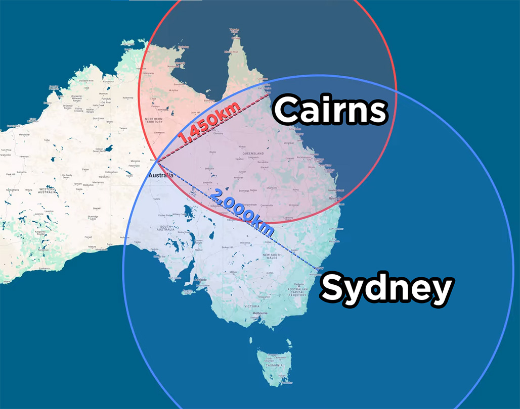
A simplified example on a large scale: imagine that I was lost somewhere in Australia, but I knew that I was exactly 2,000 km away from Sydney, and I also knew I was exactly 1,450 km away from Cairns. If I draw a 2,000 km circle around Sydney, I create a circle of possible locations I could be. If I then draw a 1,450 km circle around Cairns, I create another circle of possible places I could be. The place where these two circles overlap is where I would actually be and I would know I am in Alice Springs in the middle of Australia.
This is how our tracking system is going to work but on the scale of meters instead of kilometres. It also raises the question, how many base stations will you need? The example above is an example of tracking in 2D, and we found our location only using the equivalent of two base stations. However, if you look at the image on the right, you will see that these circles intersect in two places, meaning we could be at either of them (but we assumed I wasn't stranded in the Pacific Ocean). To eliminate this second possible location, you would need a third base station. So for 2D tracking will need a minimum of four UWB modules. One set up as the tag to be tracked, and three to act as base stations which will get measurements to the tag.
3D tracking gets a little more difficult to visualise as instead of circles of where we could possibly be, it becomes spheres. As 3D is one dimension more than 2D tracking, we will only need one more base station. So for 3D tracking, you will need a minimum of five UWB modules. One set up as the tag to be tracked, and four acting as base stations.
We say minimum here because more base stations will improve your system. If for some reason a base station loses connection (maybe you stand too close to it and block the signal, or you move the tag into one of its blindspots), your system will suddenly not have enough measurements to figure out where you are. Adding extra base stations will add extra layers of protection from this issue. By increasing the number, you may also increase the accuracy and precision of your tracking. The distance measurements from this system are accurate to within 10 cm. If you have more base stations giving more measurements, these inaccuracies can average out and give you a more accurate system.
In testing we found that adding one more base station than the minimum was very worthwhile, so we recommend it greatly. The BU03 supports up to eight base stations and all the code in this guide will support tracking with this number of stations.
What You Will Need
To follow along with this guide you will need:
- Some BU03 ultra-wideband boards. As we looked at above, for 2D tracking you will need a minimum of 4 with a recommended of 5, and for 3D tracking a minimum of 5 with a recommended 6. You can use up to a total of 9 in one system for more accurate and reliable tracking.
- A Method of powering the BU03 boards. This guide series may have you powering boards in weird and hard-to-reach places. The easiest way to power these boards is through USB-C which can be plugged into your computer or something like a phone wall charger or a phone power bank (a USB-C Raspberry Pi power supply will also work if you have some around). Longer USB-C cables can be a great help here There is also an option to power it via GPIO with either 5 V or 3.3 V. If you are using a phone power bank just be aware that some of them have power-saving modes that switch off USB power if not enough current is drawn. These boards will likely not draw enough to keep them from going into this power-saving mode, so test your power bank before committing to multiple of them.
- A Microcontroller to read and process the distance data. This guide will have code snippets for both MicroPython and C++. We will be using a Raspberry Pi Pico 2 as our MicroPython example board and an Arduino Uno R4 as our example C++ board. This guide can be adapted to work on most microcontroller boards that have dedicated UART hardware like an ESP32. Please note that the Arduino Uno R3 and older Uno boards are not suitable for this guide as they share their UART hardware with the USB serial port - you won't be able to read the UWB data and print it to your computer at the same time.
- A measuring tape to measure distances within a room. You will need to know how far away each base station is.
- A method of prototyping this all together. A breadboard and some jumper wires will suffice.
2D Spatial Tracking
Let's start by tracking a tag in 2D. If you were holding the tag, this set-up would know where abouts in a room you are standing, but not how high off the ground you are holding the tag.
Before starting this section ensure you have configured a BU03 as a tag and at least three others as base stations. We covered this in the previous guide.
First things first, we need to place our base stations, and location is going to be key here. The best tracking comes from a network of base stations that are as far apart as possible, so spread them out into the corners of the room. If you are using four stations, one in each corner is a good strategy. You will also need to balance giving them a good line of sight of the area where the tag will be tracked. It is ideal to put a base station in the corner of the room, but if something like a cupboard gives it a poor line of sight, then you may want to move it away from the corner to give it a better view of the tracking area. You are also going to want to place all of the base stations at roughly the same height - the same height the tag is going to be tracked.
Just try and mount all your base stations at roughly the same height and know that your tag will track most accurately at this height, but will still be able to track well a meter or so below or above this height.
Also keep in mind that the maximum reliable tracking distance for a base station is about 20 meters with a direct line of sight - expect less if there are obstacles in the way. If you are tracking in a large room where there may be signal dead zones, or areas where certain base stations can't get a signal, adding an extra base station or two to cover this area can help greatly. We were able to track through two separate rooms by having 2 sets of base stations in each room. If you are getting your distance data from base station 0, just be aware that if base station 0 loses contact with the tag, you will get no data, even if all the other base stations are connected. Remember, you can also get the positional data from the tag if your project calls for it (then you don't rely on always seeing base station 0).
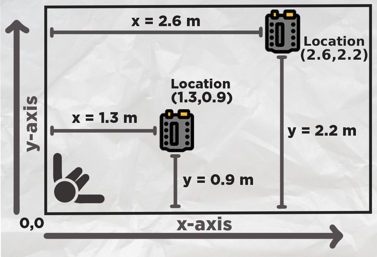
Once you have your base stations placed, we are going to need their x and y locations so we know where they are in the room. Stand in a corner of your room or area you wish to track - this is going to be your origin, or home, or zero, whatever you want to call it. This is the reference point everything is going to be measured from.
Extend out your arms along each wall. Your left arm is going to be the y-axis and your right will be your x-axis. Do not mix these up. With something like a measuring tape, measure the position of each base station in the x and y-axis from this corner. The image on the right has two example measurements.
Now that we know where our base stations are, we can input it into the following 2D tracking code. At the top you will see a section to input the (x,y) locations of all of the base stations. If you are not using that base station, set it to "None" and the code will ignore it:
from machine import UART, Pin
import time
import struct
import math

uart1 = UART(0, baudrate=115200, tx=Pin(0), rx=Pin(1))

# Base station positions (x, y) in meters
# Set to None if base station is not present
base0 = (0.0, 0.0)        # Base station 0 position
base1 = (0.0, 0.0)        # Base station 1 position
base2 = (0.0, 0.0)        # Base station 2 position
base3 = (0.0, 0.0)        # Base station 3 position
base4 = None              # Base station 4 position (leave as None if not in use)
base5 = None              # Base station 5 position (leave as None if not in use)
base6 = None              # Base station 6 position (leave as None if not in use)
base7 = None              # Base station 7 position (leave as None if not in use)

# Distance calibration offsets in meters
offset0 = 0.0
offset1 = 0.0
offset2 = 0.0
offset3 = 0.0
offset4 = 0.0
offset5 = 0.0
offset6 = 0.0
offset7 = 0.0

base_stations = [base0, base1, base2, base3, base4, base5, base6, base7]
distance_offsets = [offset0, offset1, offset2, offset3, offset4, offset5, offset6, offset7]

# Simple 2D Kalman Filter
class SimpleKalman:
    def __init__(self):
        self.state = [0.0, 0.0, 0.0, 0.0]  # x, y, vx, vy
        self.P = [
            [1.0, 0.0, 0.0, 0.0],
            [0.0, 1.0, 0.0, 0.0],
            [0.0, 0.0, 1.0, 0.0],
            [0.0, 0.0, 0.0, 1.0]
        ]
        self.Q = 0.12
        self.R = 1.1
        self.dt = 0.10
        self.initialized = False

    def predict(self):
        if not self.initialized:
            return
        new_x = self.state[0] + self.state[2] * self.dt
        new_y = self.state[1] + self.state[3] * self.dt
        new_vx = self.state[2]
        new_vy = self.state[3]
        self.state = [new_x, new_y, new_vx, new_vy]
        for i in range(4):
            for j in range(4):
                self.P[i][j] += self.Q

    def update(self, measured_x, measured_y):
        if not self.initialized:
            self.state = [measured_x, measured_y, 0.0, 0.0]
            self.initialized = True
            return measured_x, measured_y
        K_x = self.P[0][0] / (self.P[0][0] + self.R)
        K_y = self.P[1][1] / (self.P[1][1] + self.R)
        self.state[0] = self.state[0] + K_x * (measured_x - self.state[0])
        self.state[1] = self.state[1] + K_y * (measured_y - self.state[1])
        if self.dt > 0:
            self.state[2] = (self.state[0] - measured_x) / self.dt * 0.1
            self.state[3] = (self.state[1] - measured_y) / self.dt * 0.1
        self.P[0][0] = (1 - K_x) * self.P[0][0]
        self.P[1][1] = (1 - K_y) * self.P[1][1]
        return self.state[0], self.state[1]

def parse_uwb_data(data):
    """Parse UWB distance data from UART message for 8 base stations"""
    if len(data) < 35:
        return None
    if data[0] != 0xaa or data[1] != 0x25 or data[2] != 0x01:
        return None
    distances = []
    for i in range(8):
        offset = 3 + (i * 4)
        if offset + 1 < len(data):
            dist_raw = struct.unpack('<H', data[offset:offset+2])[0]
            dist_meters = dist_raw / 1000.0
            dist_calibrated = dist_meters + distance_offsets[i]
            distances.append(dist_calibrated)
        else:
            distances.append(0)
    return distances

def trilaterate_2d(positions, distances):
    """
    Perform 2D trilateration using least squares method
    Requires at least 3 valid base stations
    """
    valid_data = []
    for i, (pos, dist) in enumerate(zip(positions, distances)):
        if pos is not None and dist > 0:
            valid_data.append((pos[0], pos[1], dist))
    if len(valid_data) < 3:
        return None, None
    x1, y1, r1 = valid_data[0]
    A = []
    b = []
    for i in range(1, len(valid_data)):
        xi, yi, ri = valid_data[i]
        A.append([2*(xi - x1), 2*(yi - y1)])
        b_val = ri**2 - r1**2 - xi**2 + x1**2 - yi**2 + y1**2
        b.append(b_val)
    if len(A) >= 2:
        det = A[0][0]*A[1][1] - A[0][1]*A[1][0]
        if abs(det) < 1e-6:
            return None, None
        x = -(b[0]*A[1][1] - b[1]*A[0][1]) / det
        y = -(A[0][0]*b[1] - A[1][0]*b[0]) / det
        return x, y
    return None, None

kalman = SimpleKalman()
print("x,y,x_filtered,y_filtered,dist0,dist1,dist2,dist3,dist4,dist5,dist6,dist7")

while True:
    if uart1.any():
        try:
            message = uart1.read()
            if message:
                distances = parse_uwb_data(message)
                if distances:
                    x, y = trilaterate_2d(base_stations, distances)
                    if x is not None and y is not None:
                        kalman.predict()
                        x_filtered, y_filtered = kalman.update(x, y)
                    else:
                        kalman.predict()
                        x_filtered, y_filtered = kalman.state[0], kalman.state[1]
                    output_distances = []
                    for i, base in enumerate(base_stations):
                        if i < len(distances):
                            output_distances.append(distances[i])
                        else:
                            output_distances.append(0)
                    x_str = f"{x:.3f}" if x is not None else "0"
                    y_str = f"{y:.3f}" if y is not None else "0"
                    x_filt_str = f"{x_filtered:.3f}" if x_filtered is not None else "0"
                    y_filt_str = f"{y_filtered:.3f}" if y_filtered is not None else "0"
                    print(f"{x_str},{y_str},{x_filt_str},{y_filt_str},{output_distances[0]:.3f},{output_distances[1]:.3f},{output_distances[2]:.3f},{output_distances[3]:.3f},{output_distances[4]:.3f},{output_distances[5]:.3f},{output_distances[6]:.3f},{output_distances[7]:.3f}")
        except Exception as e:
            print(f"Error processing data: {e}")
            continue
        time.sleep(0.1)
This code is quite involved and not beginner-friendly, so we don't expect you to fully understand it, but if you are interested, we are going to quickly break it down.
Starting off, we import everything we need, set up the UART channel, and then collect all the locations of the base stations and offsets (we will look at the offsets in a bit). Then we wrap them all up in a list to make it easier to use later:
from machine import UART, Pin
import time
import struct
import math

uart1 = UART(0, baudrate=115200, tx=Pin(0), rx=Pin(1))

# Base station positions (x, y) in meters
# Set to None if base station is not present
base0 = (0.0, 0.0)        # Base station 0 position
base1 = (0.0, 0.0)        # Base station 1 position
base2 = (0.0, 0.0)        # Base station 2 position
base3 = (0.0, 0.0)        # Base station 3 position
base4 = None              # Base station 4 position (leave as None if not in use)
base5 = None              # Base station 5 position (leave as None if not in use)
base6 = None              # Base station 6 position (leave as None if not in use)
base7 = None              # Base station 7 position (leave as None if not in use)

# Distance calibration offsets in meters (positive = add to measurement, negative = subtract)
# Adjust these values to compensate for systematic measurement errors
offset0 = 0.0             # Base station 0 offset
offset1 = 0.0             # Base station 1 offset
offset2 = 0.0             # Base station 2 offset
offset3 = 0.0             # Base station 3 offset
offset4 = 0.0             # Base station 4 offset
offset5 = 0.0             # Base station 5 offset
offset6 = 0.0             # Base station 6 offset
offset7 = 0.0             # Base station 7 offset

# Put base stations and offsets in lists for easier handling
base_stations = [base0, base1, base2, base3, base4, base5, base6, base7]
distance_offsets = [offset0, offset1, offset2, offset3, offset4, offset5, offset6, offset7]
Then we define something called a Kalman filter. This is a method of smoothing out data and is the perfect sort of thing to help us get some nicer data from our tracking system. We will look at the Kalman filter in depth in a different section, as it's a great introduction to a really handy filter. Long story short though, we send it raw positional data, and it returns us smoothed and more accurate data.
# Simple 2D Kalman Filter for position and velocity
class SimpleKalman:
    def __init__(self):
        # State vector: [x, y, vx, vy] (position and velocity)
        self.state = [0.0, 0.0, 0.0, 0.0]  # x, y, vx, vy

        # State covariance matrix (4x4) - simplified diagonal
        self.P = [
            [1.0, 0.0, 0.0, 0.0],
            [0.0, 1.0, 0.0, 0.0],
            [0.0, 0.0, 1.0, 0.0],
            [0.0, 0.0, 0.0, 1.0]
        ]

        # Process noise (lower number = "I trust the previous movements more")
        self.Q = 0.12  # Simplified scalar

        # Measurement noise (lower number = "I trust the newest measurement more")
        self.R = 1.1  # Simplified scalar

        # Time step
        self.dt = 0.10  # 100ms assumed

        self.initialized = False

    def predict(self):
        if not self.initialized:
            return

        # State transition: x = x + vx*dt, y = y + vy*dt, vx = vx, vy = vy
        new_x = self.state[0] + self.state[2] * self.dt
        new_y = self.state[1] + self.state[3] * self.dt
        new_vx = self.state[2]
        new_vy = self.state[3]

        self.state = [new_x, new_y, new_vx, new_vy]

        # Update covariance (simplified)
        for i in range(4):
            for j in range(4):
                self.P[i][j] += self.Q

    def update(self, measured_x, measured_y):
        if not self.initialized:
            # Initialize with first measurement
            self.state = [measured_x, measured_y, 0.0, 0.0]
            self.initialized = True
            return measured_x, measured_y

        # Kalman gain (simplified for position measurements only)
        K_x = self.P[0][0] / (self.P[0][0] + self.R)
        K_y = self.P[1][1] / (self.P[1][1] + self.R)

        # Update state with measurement
        self.state[0] = self.state[0] + K_x * (measured_x - self.state[0])
        self.state[1] = self.state[1] + K_y * (measured_y - self.state[1])

        # Update velocity estimates
        if self.dt > 0:
            self.state[2] = (self.state[0] - measured_x) / self.dt * 0.1  # Simplified velocity update
            self.state[3] = (self.state[1] - measured_y) / self.dt * 0.1

        # Update covariance (simplified)
        self.P[0][0] = (1 - K_x) * self.P[0][0]
        self.P[1][1] = (1 - K_y) * self.P[1][1]

        return self.state[0], self.state[1]
Next we define a parser function. This is pretty much the same as the demo code from the previous guide, it takes in the raw 16-bit little-endian values coming from the UART, and outputs nice and human readable numbers.
def parse_uwb_data(data):
    """Parse UWB distance data from UART message for 8 base stations"""
    if len(data) < 35:  # Minimum expected length for 8 stations
        return None

    # Check for start byte \xaa%\x01
    if data[0] != 0xaa or data[1] != 0x25 or data[2] != 0x01:
        return None

    # Extract 8 distance values (16-bit little-endian, starting at byte 3)
    distances = []
    for i in range(8):
        offset = 3 + (i * 4)  # Each distance is 4 bytes apart
        if offset + 1 < len(data):
            # Unpack as little-endian 16-bit unsigned integer
            dist_raw = struct.unpack('
Then we create a function to perform our trilateration. From our explanation at the start, each base station is going to measure the distance from itself to the tag. You can then use this distance to draw a circle around each base station of possible locations where the tag is. Where all of the base stations' circles overlap is where the tag likely is. This function is just a mathematical way to determine the location where those circles overlap. This uses something called the least squares method which is a really common method of finding truth from conflicting data or measurements.
def trilaterate_2d(positions, distances):
    """
    Perform 2D trilateration using least squares method
    positions: list of (x, y) tuples for base stations
    distances: list of distances to each base station
    Requires at least 3 valid base stations for positioning
    """
    # Filter out base stations that are None or have 0 distance
    valid_data = []
    for i, (pos, dist) in enumerate(zip(positions, distances)):
        if pos is not None and dist > 0:
            valid_data.append((pos[0], pos[1], dist))

    if len(valid_data) < 3:
        return None, None  # Need at least 3 points for reliable 2D positioning

    # Use least squares method with 3+ points
    # Set up system of equations for least squares
    # (x - xi)² + (y - yi)² = ri²
    # Linearize: x² - 2*xi*x + xi² + y² - 2*yi*y + yi² = ri²
    # Rearrange: -2*xi*x - 2*yi*y = ri² - x² - y² - xi² - yi²

    # Use first point as reference
    x1, y1, r1 = valid_data[0]

    A = []
    b = []

    for i in range(1, len(valid_data)):
        xi, yi, ri = valid_data[i]

        # Coefficient matrix row: [2*(xi - x1), 2*(yi - y1)]
        A.append([2 * (xi - x1), 2 * (yi - y1)])

        # Right side: ri² - r1² - xi² + x1² - yi² + y1²
        b_val = ri**2 - r1**2 - xi**2 + x1**2 - yi**2 + y1**2
        b.append(b_val)

    # Solve using simple 2x2 system if we have exactly 3 points
    if len(A) >= 2:
        # Take first 2 equations for 2x2 system
        det = A[0][0] * A[1][1] - A[0][1] * A[1][0]

        if abs(det) < 1e-6:  # Nearly singular
            return None, None

        # Solve for [x, y]
        x = -(b[0] * A[1][1] - b[1] * A[0][1]) / det
        y = -(A[0][0] * b[1] - A[1][0] * b[0]) / det

        return x, y

    return None, None
Then we finally get to our loop where we start to use these functions. Our loop begins by reading data from our UART channel and if there is a message, it will receive it and run it through the parser function to get nice readable numbers out of it:
while True:
    if uart1.any():
        try:
            message = uart1.read()
            if message:
                distances = parse_uwb_data(message)
Next, if it gets valid distance measurements, it will send all of those readings to the trilaterate function, as well as all the positions of the base stations. The trilaterate function will return where it thinks the tag is with an x and y coordinate. This coordinate will use the same system of measurements you used to get the location of each base station.
                if distances:
                    # Perform trilateration
                    x, y = trilaterate_2d(base_stations, distances)
If the trilateration function is successful, we take the raw data from it and run it through the Kalman filter. This raw data can be jittery and may bounce around quite a lot - the Kalman will smooth it out.
                    if x is not None and y is not None:
                        # Predict next state
                        kalman.predict()

                        # Update with measurement
                        x_filtered, y_filtered = kalman.update(x, y)
                    else:
                        # No valid position, just predict
                        kalman.predict()
                        x_filtered, y_filtered = kalman.state[0], kalman.state[1]
Then the rest of the code deals with printing and outputting the data in something called a CSV format, which is something we will use later in the visualisation section. If you wish to adapt this code to your own project, you can put your custom code here. X and y will give you the jittery, raw readings, and x_filtered and y_filtered will give you the nicer, smoothed data. The code has a 0.1-second sleep in it. You must not change the sleep time here, as the Kalman filter is set up to run on this sleep time. If you do change this, you will need to change it in the Kalman filter as well - more on this later.
                    # Prepare output distances (0 if base station not present)
                    output_distances = []
                    for i, base in enumerate(base_stations):
                        if i < len(distances):
                            output_distances.append(distances[i])
                        else:
                            output_distances.append(0)


                    # If you are adapting this to your own code, you can use the values x_filtered and y_filtered to get the estimated
                    # x and y location of the tag. Or you can get just use x and y to get the raw, unfiltered, more jittery data.

                    # Format position values
                    x_str = f"{x:.3f}" if x is not None else "0"
                    y_str = f"{y:.3f}" if y is not None else "0"
                    x_filt_str = f"{x_filtered:.3f}" if x_filtered is not None else "0"
                    y_filt_str = f"{y_filtered:.3f}" if y_filtered is not None else "0"

                    # Print CSV line with both raw and filtered positions and all 8 distances
                    print(f"{x_str},{y_str},{x_filt_str},{y_filt_str},{output_distances[0]:.3f},{output_distances[1]:.3f},{output_distances[2]:.3f},{output_distances[3]:.3f},{output_distances[4]:.3f},{output_distances[5]:.3f},{output_distances[6]:.3f},{output_distances[7]:.3f}")

        except Exception as e:
            print(f"Error processing data: {e}")
            continue

        time.sleep(0.1)  # a 100ms timestep - important for kalman
Now that we know where our base stations are, we can input it into the following 2D tracking code. At the top you will see a section to input the (x,y) locations of all of the base stations. If you are not using that base station, set it to "NULL" and the code will ignore it:
#include// Base station positions (x, y) in meters // Set to NULL if base station is not present struct Position { float x, y; }; Position* base0 = new Position{1.2, 2.9}; // Base station 0 position Position* base1 = new Position{3.12, 2.96}; // Base station 1 position Position* base2 = new Position{0, 1.1}; // Base station 2 position Position* base3 = new Position{3.08, 0.0}; // Base station 3 position Position* base4 = NULL; // Base station 4 position (leave as NULL if not in use) Position* base5 = NULL; // Base station 5 position (leave as NULL if not in use) Position* base6 = NULL; // Base station 6 position (leave as NULL if not in use) Position* base7 = NULL; // Base station 7 position (leave as NULL if not in use) // Distance calibration offsets in meters (positive = add to measurement, negative = subtract) // Adjust these values to compensate for systematic measurement errors float offset0 = 0.0; // Base station 0 offset float offset1 = 0.0; // Base station 1 offset float offset2 = 0.0; // Base station 2 offset float offset3 = 0.0; // Base station 3 offset float offset4 = 0.0; // Base station 4 offset float offset5 = 0.0; // Base station 5 offset float offset6 = 0.0; // Base station 6 offset float offset7 = 0.0; // Base station 7 offset // Put base stations and offsets in arrays for easier handling Position* base_stations[8] = {base0, base1, base2, base3, base4, base5, base6, base7}; float distance_offsets[8] = {offset0, offset1, offset2, offset3, offset4, offset5, offset6, offset7}; // Simple 2D Kalman Filter for position and velocity class SimpleKalman { private: float state[4]; // [x, y, vx, vy] float P[4][4]; // State covariance matrix float Q; // Process noise float R; // Measurement noise float dt; // Time step bool initialized; public: SimpleKalman() { // Initialize state vector state[0] = 0.0; state[1] = 0.0; state[2] = 0.0; state[3] = 0.0; // Initialize covariance matrix for (int i = 0; i < 4; i++) { for (int j = 0; j < 4; j++) { P[i][j] = (i == j) ? 1.0 : 0.0; } } Q = 0.12; // Process noise R = 1.1; // Measurement noise dt = 0.10; // Time step initialized = false; } void predict() { if (!initialized) return; // State transition: x = x + vx*dt, y = y + vy*dt, vx = vx, vy = vy float new_x = state[0] + state[2] * dt; float new_y = state[1] + state[3] * dt; float new_vx = state[2]; float new_vy = state[3]; state[0] = new_x; state[1] = new_y; state[2] = new_vx; state[3] = new_vy; // Update covariance (simplified) for (int i = 0; i < 4; i++) { for (int j = 0; j < 4; j++) { P[i][j] += Q; } } } void update(float measured_x, float measured_y, float* filtered_x, float* filtered_y) { if (!initialized) { // Initialize with first measurement state[0] = measured_x; state[1] = measured_y; state[2] = 0.0; state[3] = 0.0; initialized = true; *filtered_x = measured_x; *filtered_y = measured_y; return; } // Kalman gain (simplified for position measurements only) float K_x = P[0][0] / (P[0][0] + R); float K_y = P[1][1] / (P[1][1] + R); // Update state with measurement state[0] = state[0] + K_x * (measured_x - state[0]); state[1] = state[1] + K_y * (measured_y - state[1]); // Update velocity estimates if (dt > 0) { state[2] = (state[0] - measured_x) / dt * 0.1; // Simplified velocity update state[3] = (state[1] - measured_y) / dt * 0.1; } // Update covariance (simplified) P[0][0] = (1 - K_x) * P[0][0]; P[1][1] = (1 - K_y) * P[1][1]; *filtered_x = state[0]; *filtered_y = state[1]; } void getCurrentState(float* x, float* y) { *x = state[0]; *y = state[1]; } }; SimpleKalman kalman; bool parseUwbData(uint8_t* data, int dataLen, float* distances) { if (dataLen < 35) { return false; } // Check for start byte if (data[0] != 0xaa || data[1] != 0x25 || data[2] != 0x01) { return false; } // Extract 8 distance values (16-bit little-endian, starting at byte 3) for (int i = 0; i < 8; i++) { int offset = 3 + (i * 4); // Each distance is 4 bytes apart if (offset + 1 < dataLen) { // Unpack as little-endian 16-bit unsigned integer uint16_t dist_raw = data[offset] | (data[offset + 1] << 8); // Convert to meters float dist_meters = dist_raw / 1000.0; // Apply calibration offset for this station distances[i] = dist_meters + distance_offsets[i]; } else { distances[i] = 0; } } return true; } bool trilaterate2d(float* distances, float* x, float* y) { // Filter out base stations that are NULL or have 0 distance struct ValidData { float x, y, dist; }; ValidData valid_data[8]; int valid_count = 0; for (int i = 0; i < 8; i++) { if (base_stations[i] != NULL && distances[i] > 0) { valid_data[valid_count].x = base_stations[i]->x; valid_data[valid_count].y = base_stations[i]->y; valid_data[valid_count].dist = distances[i]; valid_count++; } } if (valid_count < 3) { return false; // Need at least 3 points for reliable 2D positioning } // Use least squares method with 3+ points // Use first point as reference float x1 = valid_data[0].x; float y1 = valid_data[0].y; float r1 = valid_data[0].dist; // Build coefficient matrix A and vector b float A[7][2]; // Maximum 7 equations (8-1 base stations) float b[7]; int eq_count = 0; for (int i = 1; i < valid_count && eq_count < 7; i++) { float xi = valid_data[i].x; float yi = valid_data[i].y; float ri = valid_data[i].dist; // Coefficient matrix row: [2*(xi - x1), 2*(yi - y1)] A[eq_count][0] = 2 * (xi - x1); A[eq_count][1] = 2 * (yi - y1); // Right side: ri² - r1² - xi² + x1² - yi² + y1² b[eq_count] = ri*ri - r1*r1 - xi*xi + x1*x1 - yi*yi + y1*y1; eq_count++; } // Solve using simple 2x2 system if we have at least 2 equations if (eq_count >= 2) { // Take first 2 equations for 2x2 system float det = A[0][0] * A[1][1] - A[0][1] * A[1][0]; if (abs(det) < 1e-6) { // Nearly singular return false; } // Solve for [x, y] *x = -(b[0] * A[1][1] - b[1] * A[0][1]) / det; *y = -(A[0][0] * b[1] - A[1][0] * b[0]) / det; return true; } return false; } void setup() { Serial.begin(115200); Serial1.begin(115200); Serial.println("x,y,x_filtered,y_filtered,dist0,dist1,dist2,dist3,dist4,dist5,dist6,dist7"); } void loop() { static uint8_t buffer[256]; static int bufferIndex = 0; static bool messageStarted = false; // Check if anything is available in buffer while (Serial1.available()) { uint8_t incomingByte = Serial1.read(); // Look for start of message if (!messageStarted && incomingByte == 0xAA) { messageStarted = true; bufferIndex = 0; buffer[bufferIndex++] = incomingByte; } else if (messageStarted) { buffer[bufferIndex++] = incomingByte; // Check if we have a complete message (35+ bytes expected) if (bufferIndex >= 35) { float distances[8]; if (parseUwbData(buffer, bufferIndex, distances)) { // Perform trilateration float x, y; bool validPosition = trilaterate2d(distances, &x, &y); float x_filtered, y_filtered; // Apply Kalman filtering if we have a valid position if (validPosition) { // Predict next state kalman.predict(); // Update with measurement kalman.update(x, y, &x_filtered, &y_filtered); } else { // No valid position, just predict kalman.predict(); kalman.getCurrentState(&x_filtered, &y_filtered); } // Format position values String x_str = validPosition ? String(x, 3) : "0"; String y_str = validPosition ? String(y, 3) : "0"; String x_filt_str = String(x_filtered, 3); String y_filt_str = String(y_filtered, 3); // Print CSV line with both raw and filtered positions and all 8 distances Serial.print(x_str); Serial.print(","); Serial.print(y_str); Serial.print(","); Serial.print(x_filt_str); Serial.print(","); Serial.print(y_filt_str); Serial.print(","); Serial.print(distances[0], 3); Serial.print(","); Serial.print(distances[1], 3); Serial.print(","); Serial.print(distances[2], 3); Serial.print(","); Serial.print(distances[3], 3); Serial.print(","); Serial.print(distances[4], 3); Serial.print(","); Serial.print(distances[5], 3); Serial.print(","); Serial.print(distances[6], 3); Serial.print(","); Serial.print(distances[7], 3); Serial.println(); } // Reset for next message messageStarted = false; bufferIndex = 0; } // Prevent buffer overflow if (bufferIndex >= 256) { messageStarted = false; bufferIndex = 0; } } } delay(100); }
Run this code, power on all your base stations, and you should see some numbers being printed to the serial monitor like in the image on the right! The first two numbers are the raw x and y location data, the third and fourth numbers are the filtered x and y data, and the following eight numbers are the raw distance readings from each base station to the tag. And with this, you are tracking the tag in 2d space!
If your tracking is a bit inaccurate, you may need to calibrate your base stations to account for their offsets. As we mentioned last guide, each base station may read 10cm to 20cm too high or low. If you are tracking a tag in a large room, this offset might not give you any hassle. But in a smaller room, especially when the tag is close to a base station, you may get some dodgy data.
To calibrate the offset, simply hold the tag at a known distance, then see what distance it actually reads and enter the offset value in the offset section of the code. For example, I held the tag 2 meters away from base station 3, and found that it read about 2.15 meters. I then entered -0.15 into the offset section to account for this error. I found that base station 6, on the other hand, read 1.82 meters when it should be 2 meters. I input 0.18 in the offset section to fix this. After doing so, tracking was improved.
![]()
Processing IDE Visualisation
Let's now visualise this tracking as it is just plain cool to see, and will greatly help us use this system as a visualisation is more "human-brain-friendly" than numbers being printed out. To do so, we will be using Processing IDE, a free and open-source program that is fantastic at drawing visuals like this. Download Processing IDE and paste in the following code:
import processing.serial.*;

// Serial communication
Serial myPort;
String inString = "";

// Base station positions (x, y) in meters (set to null if unused)
float[] base0 = {0.0, 0.0};
float[] base1 = {0.0, 0.0};
float[] base2 = {0.0, 0.0};
float[] base3 = {0.0, 0.0};
float[] base4 = null;
float[] base5 = null;
float[] base6 = null;
float[] base7 = null;

// Put base stations in array (null for unused stations)
float[][] baseStations = {base0, base1, base2, base3, base4, base5, base6, base7};

// Visualization bounds (in meters)
float minX = -0.5;
float maxX = 6;
float minY = -0.5;
float maxY = 3.5;

// Current data
float tagX = 0;
float tagY = 0;
float tagXFiltered = 0;
float tagYFiltered = 0;
float[] distances = new float[8];
boolean dataReceived = false;

// Colors for base stations
color[] baseColors = {
  color(255, 0, 0),    // Red
  color(0, 255, 0),    // Green
  color(0, 0, 255),    // Blue
  color(255, 255, 0),  // Yellow
  color(255, 0, 255),  // Magenta
  color(0, 255, 255),  // Cyan
  color(255, 128, 0),  // Orange
  color(128, 0, 255)   // Purple
};

void setup() {
  size(1600, 900);
  println("Available serial ports:");
  printArray(Serial.list());

  String portName = Serial.list()[0]; // adjust as needed
  myPort = new Serial(this, "COM9", 115200);
  myPort.bufferUntil('\n');

  background(0);
}

void draw() {
  background(0);

  drawCoordinateSystem();

  if (dataReceived) {
    for (int i = 0; i < baseStations.length; i++) {
      if (baseStations[i] != null) {
        drawBaseStation(i, baseStations[i][0], baseStations[i][1], distances[i]);
      }
    }

    drawTagPosition(tagX, tagY, "RAW", color(255, 100, 100));
    drawTagPosition(tagXFiltered, tagYFiltered, "FILTERED", color(100, 255, 100));
  }

  drawLegend();
}

void drawCoordinateSystem() {
  stroke(50);
  strokeWeight(1);
  for (float x = minX; x <= maxX; x += 0.5) {
    float screenX = map(x, minX, maxX, 50, width - 50);
    line(screenX, 50, screenX, height - 50);
  }
  for (float y = minY; y <= maxY; y += 0.5) {
    float screenY = map(y, minY, maxY, height - 50, 50);
    line(50, screenY, width - 50, screenY);
  }
  stroke(100);
  strokeWeight(2);
  float originX = map(0, minX, maxX, 50, width - 50);
  float originY = map(0, minY, maxY, height - 50, 50);
  line(originX, 50, originX, height - 50);
  line(50, originY, width - 50, originY);

  fill(255);
  textAlign(CENTER);
  text("X (meters)", width/2, height - 20);
  pushMatrix();
  translate(20, height/2);
  rotate(-PI/2);
  text("Y (meters)", 0, 0);
  popMatrix();
}

void drawBaseStation(int index, float x, float y, float distance) {
  float screenX = map(x, minX, maxX, 50, width - 50);
  float screenY = map(y, minY, maxY, height - 50, 50);

  if (distance > 0) {
    stroke(baseColors[index]);
    strokeWeight(1);
    fill(baseColors[index], 30);
    float radius = map(distance, 0, maxX - minX, 0, width - 100);
    ellipse(screenX, screenY, radius*2, radius*2);
  }

  stroke(baseColors[index]);
  strokeWeight(3);
  fill(baseColors[index]);
  ellipse(screenX, screenY, 12, 12);

  fill(255);
  textAlign(CENTER);
  text("B" + index, screenX, screenY - 15);

  if (distance > 0) {
    text(nf(distance, 1, 2) + "m", screenX, screenY + 25);
  }
}

void drawTagPosition(float x, float y, String label, color c) {
  float screenX = map(x, minX, maxX, 50, width - 50);
  float screenY = map(y, minY, maxY, height - 50, 50);
  stroke(c);
  strokeWeight(2);
  fill(c);
  ellipse(screenX, screenY, 12, 12);
  line(screenX - 8, screenY, screenX + 8, screenY);
  line(screenX, screenY - 8, screenX, screenY + 8);
  fill(c);
  textAlign(CENTER);
  text(label, screenX, screenY - 15);
  text("(" + nf(x, 1, 2) + ", " + nf(y, 1, 2) + ")", screenX, screenY + 25);
}

void drawLegend() {
  fill(255);
  textAlign(LEFT);
  text("Legend:", 10, 20);
  int y = 40;
  for (int i = 0; i < baseStations.length; i++) {
    if (baseStations[i] != null) {
      fill(baseColors[i]);
      ellipse(25, y, 8, 8);
      fill(255);
      text("Base Station " + i, 35, y+5);
      y += 20;
    }
  }
  fill(255, 100, 100);
  ellipse(25, y, 8, 8);
  fill(255);
  text("Raw Position", 35, y+5);
  y += 20;
  fill(100, 255, 100);
  ellipse(25, y, 8, 8);
  fill(255);
  text("Filtered Position", 35, y+5);
}

void serialEvent(Serial myPort) {
  inString = myPort.readStringUntil('\n');
  if (inString != null) {
    inString = trim(inString);
    if (inString.startsWith("x,y,x_filtered")) return;

    String[] data = split(inString, ',');
    if (data.length >= 12) {
      try {
        tagX = float(data[0]);
        tagY = float(data[1]);
        tagXFiltered = float(data[2]);
        tagYFiltered = float(data[3]);
        for (int i = 0; i < 8; i++) {
          distances[i] = float(data[4 + i]);
        }
        dataReceived = true;
      } catch (Exception e) {
        println("Parse error: " + inString);
      }
    }
  }
}
This code is going to take in the CSV-formatted information the microcontroller is printing out, and draw it in a top-down view of your tracking area. Before you run it, you will need to modify a few things. First of all, you need to tell it the locations of your base stations. This is the same process as before, and you will find the section to input these numbers at the top of the code. Do note that the processing IDE uses curly brackets, and if a base station is not present, it will need to be set as null - just ensure you follow the format already in the demo code.
Under that section, you will also find four variables you will need to modify to define the area you want the visualisation to track. minX and maxX define the size of the room in the x-axis you want to track (in meters), while minY and maxY define it in the y-axis. Have a play around with these values, and if you are unsure what to do, leave minx and miny at -0.5 and set maxX and maxY to the size of your room.
The final thing you will need to do is input the COM Port your microcontroller is using. You can find this easily through Your IDE. You will find the section you need to change at about line 52 and in the demo code it is COM Port 9 as an example.
With all those changes, we are ready to run this code. Before doing so, close the program you used to code your microcontroller (e.g. Thonny or Arduino IDE). They will likely already be connected to the COM Port of your microcontroller, which will prevent Processing IDE from connecting to it. Once it is closed, unplug and replug in your microcontroller and run the processing code.
You should be greeted with a visualisation like the image on the right. You will be able to see the location of each base station, and the ring around each is the measured distance to the tag (our circle of potential locations). The raw jittery data will be visualised by the red dot, and the green dot that lags behind it is the smoothed data through the Kalman filter. We will look at how to tune this filter in a bit to be more or less responsive.
And with that, we have a nice jump-off point for your project! You now have a series of base stations and the code required to track an object in 2D space, which is a pretty powerful tool to add to a maker project. If you want to take this to the next level though, tracking in 3D space is not much more work than 2D...
![]()
3D Spatial Tracking
Let's now take a look at how to track a tag in 3 3-dimensional space. This is going to be largely the same process as our 2D tracking setup, just with different code and a few additional things. Starting off, we will need to place our base stations in some new locations (also remember we need a minimum of 4 base stations now). The same wisdom as 2D tracking applies now, but we are also going to want some to be placed as high as possible, and some as low as possible. With eight base stations, the ideal set-up is to place one each four corners of the floor, and four corners of the ceiling. This gave us some really solid tracking with plenty of redundancy.
You will also need to get the x,y, and z coordinates of each base station. You can get the x and the y distances with the exact same method as before, and the new z-axis is just going to be a measurement of how high off the ground the base station is. Insert these values into the new 3D tracking code:
from machine import UART, Pin
import time
import struct
import math

uart1 = UART(0, baudrate=115200, tx=Pin(0), rx=Pin(1))

# Base station positions (x, y, z) in meters
base0 = (1.95, 3.1, 0.99)
base1 = (3.03, 0.56, 0.12)
base2 = (3.53, 2.43, 1.48)
base3 = (0.0, 0.34, 2.24)
base4 = (0.98, 3.12, 2.09)
base5 = None
base6 = None
base7 = None

# Distance calibration offsets in meters
offset0 = 0.0
offset1 = 0.0
offset2 = 0.0
offset3 = 0.0
offset4 = 0.0
offset5 = 0.0
offset6 = 0.0
offset7 = 0.0

base_stations = [base0, base1, base2, base3, base4, base5, base6, base7]
distance_offsets = [offset0, offset1, offset2, offset3, offset4, offset5, offset6, offset7]

class SimpleKalman3D:
    def __init__(self):
        self.state = [0.0] * 6  # x, y, z, vx, vy, vz
        self.P = [[1.0 if i == j else 0.0 for j in range(6)] for i in range(6)]
        self.Q = 0.12
        self.R = 1.1
        self.dt = 0.10
        self.initialized = False

    def predict(self):
        if not self.initialized:
            return
        self.state[0] += self.state[3] * self.dt
        self.state[1] += self.state[4] * self.dt
        self.state[2] += self.state[5] * self.dt
        for i in range(6):
            for j in range(6):
                self.P[i][j] += self.Q

    def update(self, mx, my, mz):
        if not self.initialized:
            self.state = [mx, my, mz, 0.0, 0.0, 0.0]
            self.initialized = True
            return mx, my, mz
        Kx = self.P[0][0] / (self.P[0][0] + self.R)
        Ky = self.P[1][1] / (self.P[1][1] + self.R)
        Kz = self.P[2][2] / (self.P[2][2] + self.R)
        self.state[0] += Kx * (mx - self.state[0])
        self.state[1] += Ky * (my - self.state[1])
        self.state[2] += Kz * (mz - self.state[2])
        if self.dt > 0:
            self.state[3] = (self.state[0] - mx) / self.dt * 0.1
            self.state[4] = (self.state[1] - my) / self.dt * 0.1
            self.state[5] = (self.state[2] - mz) / self.dt * 0.1
        self.P[0][0] *= (1 - Kx)
        self.P[1][1] *= (1 - Ky)
        self.P[2][2] *= (1 - Kz)
        return self.state[0], self.state[1], self.state[2]

def parse_uwb_data(data):
    if len(data) < 35 or data[0] != 0xaa or data[1] != 0x25 or data[2] != 0x01:
        return None
    distances = []
    for i in range(8):
        offset = 3 + (i * 4)
        if offset + 1 < len(data):
            dist_raw = struct.unpack('<H', data[offset:offset+2])[0]
            dist_m = dist_raw / 1000.0
            dist_calibrated = dist_m + distance_offsets[i]
            distances.append(dist_calibrated)
        else:
            distances.append(0)
    return distances

def trilaterate_3d(positions, distances):
    valid = []
    for i, (pos, dist) in enumerate(zip(positions, distances)):
        if pos is not None and dist > 0:
            valid.append((pos[0], pos[1], pos[2], dist))
    if len(valid) < 4:
        return None, None, None
    x1, y1, z1, r1 = valid[0]
    A = []
    b = []
    for i in range(1, len(valid)):
        xi, yi, zi, ri = valid[i]
        A.append([2*(xi - x1), 2*(yi - y1), 2*(zi - z1)])
        b_val = (xi**2 - x1**2) + (yi**2 - y1**2) + (zi**2 - z1**2) + (r1**2 - ri**2)
        b.append(b_val)
    if len(A) < 3:
        return None, None, None
    # Solve 3x3 system using Cramer's Rule
    def det3(m):
        return (m[0][0]*(m[1][1]*m[2][2] - m[1][2]*m[2][1])
              - m[0][1]*(m[1][0]*m[2][2] - m[1][2]*m[2][0])
              + m[0][2]*(m[1][0]*m[2][1] - m[1][1]*m[2][0]))
    M = A[:3]
    det_main = det3(M)
    if abs(det_main) < 1e-6:
        return None, None, None
    def replace_column(matrix, col_idx, new_col):
        return [[new_col[row] if col == col_idx else matrix[row][col] for col in range(3)] for row in range(3)]
    x = det3(replace_column(M, 0, b[:3])) / det_main
    y = det3(replace_column(M, 1, b[:3])) / det_main
    z = det3(replace_column(M, 2, b[:3])) / det_main
    return x, y, z

kalman = SimpleKalman3D()
print("x,y,z,x_filtered,y_filtered,z_filtered,dist0,dist1,dist2,dist3,dist4,dist5,dist6,dist7")

while True:
    if uart1.any():
        try:
            message = uart1.read()
            if message:
                distances = parse_uwb_data(message)
                if distances:
                    x, y, z = trilaterate_3d(base_stations, distances)
                    if x is not None and y is not None and z is not None:
                        kalman.predict()
                        x_filt, y_filt, z_filt = kalman.update(x, y, z)
                    else:
                        kalman.predict()
                        x_filt, y_filt, z_filt = kalman.state[0], kalman.state[1], kalman.state[2]
                    x_str = f"{x:.3f}" if x is not None else "0"
                    y_str = f"{y:.3f}" if y is not None else "0"
                    z_str = f"{z:.3f}" if z is not None else "0"
                    x_filt_str = f"{x_filt:.3f}"
                    y_filt_str = f"{y_filt:.3f}"
                    z_filt_str = f"{z_filt:.3f}"
                    dist_strs = [f"{d:.3f}" for d in distances]
                    print(f"{x_str},{y_str},{z_str},{x_filt_str},{y_filt_str},{z_filt_str}," + ",".join(dist_strs))
        except Exception as e:
            print(f"Error processing data: {e}")
            continue
        time.sleep(0.095)  # ~100ms timestep
#include// Base station positions (x, y, z) in meters // Set to NULL if base station is not present struct Position3D { float x, y, z; }; Position3D* base0 = new Position3D{1.2, 2.9, 0.72}; // Base station 0 position Position3D* base1 = new Position3D{3.12, 2.96, 1.53}; // Base station 1 position Position3D* base2 = new Position3D{0, 1.1, 2.25}; // Base station 2 position Position3D* base3 = new Position3D{3.08, 0.0, 1.36}; // Base station 3 position Position3D* base4 = NULL; // Base station 4 position (leave as NULL if not in use) Position3D* base5 = NULL; // Base station 5 position (leave as NULL if not in use) Position3D* base6 = NULL; // Base station 6 position (leave as NULL if not in use) Position3D* base7 = NULL; // Base station 7 position (leave as NULL if not in use) #include // Distance calibration offsets in meters (positive = add to measurement, negative = subtract) // Adjust these values to compensate for systematic measurement errors float offset0 = 0.0; // Base station 0 offset float offset1 = 0.0; // Base station 1 offset float offset2 = 0.0; // Base station 2 offset float offset3 = 0.0; // Base station 3 offset float offset4 = 0.0; // Base station 4 offset float offset5 = 0.0; // Base station 5 offset float offset6 = 0.0; // Base station 6 offset float offset7 = 0.0; // Base station 7 offset // Put base stations and offsets in arrays for easier handling Position3D* base_stations[8] = {base0, base1, base2, base3, base4, base5, base6, base7}; float distance_offsets[8] = {offset0, offset1, offset2, offset3, offset4, offset5, offset6, offset7}; // Simple 3D Kalman Filter for position and velocity class SimpleKalman3D { private: float state[6]; // [x, y, z, vx, vy, vz] float P[6][6]; // State covariance matrix float Q; // Process noise float R; // Measurement noise float dt; // Time step bool initialized; public: SimpleKalman3D() { // Initialize state vector for (int i = 0; i < 6; i++) { state[i] = 0.0; } // Initialize covariance matrix for (int i = 0; i < 6; i++) { for (int j = 0; j < 6; j++) { P[i][j] = (i == j) ? 1.0 : 0.0; } } Q = 0.12; // Process noise R = 1.1; // Measurement noise dt = 0.10; // Time step initialized = false; } void predict() { if (!initialized) return; // State transition: x = x + vx*dt, y = y + vy*dt, z = z + vz*dt, vx = vx, vy = vy, vz = vz float new_x = state[0] + state[3] * dt; float new_y = state[1] + state[4] * dt; float new_z = state[2] + state[5] * dt; float new_vx = state[3]; float new_vy = state[4]; float new_vz = state[5]; state[0] = new_x; state[1] = new_y; state[2] = new_z; state[3] = new_vx; state[4] = new_vy; state[5] = new_vz; // Update covariance (simplified) for (int i = 0; i < 6; i++) { for (int j = 0; j < 6; j++) { P[i][j] += Q; } } } void update(float measured_x, float measured_y, float measured_z, float* filtered_x, float* filtered_y, float* filtered_z) { if (!initialized) { // Initialize with first measurement state[0] = measured_x; state[1] = measured_y; state[2] = measured_z; state[3] = 0.0; state[4] = 0.0; state[5] = 0.0; initialized = true; *filtered_x = measured_x; *filtered_y = measured_y; *filtered_z = measured_z; return; } // Kalman gain (simplified for position measurements only) float K_x = P[0][0] / (P[0][0] + R); float K_y = P[1][1] / (P[1][1] + R); float K_z = P[2][2] / (P[2][2] + R); // Update state with measurement state[0] = state[0] + K_x * (measured_x - state[0]); state[1] = state[1] + K_y * (measured_y - state[1]); state[2] = state[2] + K_z * (measured_z - state[2]); // Update velocity estimates if (dt > 0) { state[3] = (state[0] - measured_x) / dt * 0.1; // Simplified velocity update state[4] = (state[1] - measured_y) / dt * 0.1; state[5] = (state[2] - measured_z) / dt * 0.1; } // Update covariance (simplified) P[0][0] = (1 - K_x) * P[0][0]; P[1][1] = (1 - K_y) * P[1][1]; P[2][2] = (1 - K_z) * P[2][2]; *filtered_x = state[0]; *filtered_y = state[1]; *filtered_z = state[2]; } void getCurrentState(float* x, float* y, float* z) { *x = state[0]; *y = state[1]; *z = state[2]; } }; SimpleKalman3D kalman; bool parseUwbData(uint8_t* data, int dataLen, float* distances) { if (dataLen < 35) { return false; } // Check for start byte if (data[0] != 0xaa || data[1] != 0x25 || data[2] != 0x01) { return false; } // Extract 8 distance values (16-bit little-endian, starting at byte 3) for (int i = 0; i < 8; i++) { int offset = 3 + (i * 4); // Each distance is 4 bytes apart if (offset + 1 < dataLen) { // Unpack as little-endian 16-bit unsigned integer uint16_t dist_raw = data[offset] | (data[offset + 1] << 8); // Convert to meters float dist_meters = dist_raw / 1000.0; // Apply calibration offset for this station distances[i] = dist_meters + distance_offsets[i]; } else { distances[i] = 0; } } return true; } bool trilaterate3d(float* distances, float* x, float* y, float* z) { // Filter out base stations that are NULL or have 0 distance struct ValidData3D { float x, y, z, dist; }; ValidData3D valid_data[8]; int valid_count = 0; for (int i = 0; i < 8; i++) { if (base_stations[i] != NULL && distances[i] > 0) { valid_data[valid_count].x = base_stations[i]->x; valid_data[valid_count].y = base_stations[i]->y; valid_data[valid_count].z = base_stations[i]->z; valid_data[valid_count].dist = distances[i]; valid_count++; } } if (valid_count < 4) { return false; // Need at least 4 points for reliable 3D positioning } // Use least squares method with 4+ points // Use first point as reference float x1 = valid_data[0].x; float y1 = valid_data[0].y; float z1 = valid_data[0].z; float r1 = valid_data[0].dist; // Build coefficient matrix A and vector b for overdetermined system float A[7][3]; // Maximum 7 equations (8-1 base stations) float b[7]; int eq_count = 0; for (int i = 1; i < valid_count && eq_count < 7; i++) { float xi = valid_data[i].x; float yi = valid_data[i].y; float zi = valid_data[i].z; float ri = valid_data[i].dist; // Coefficient matrix row: [2*(xi - x1), 2*(yi - y1), 2*(zi - z1)] A[eq_count][0] = 2 * (xi - x1); A[eq_count][1] = 2 * (yi - y1); A[eq_count][2] = 2 * (zi - z1); // Right side: xi² - x1² + yi² - y1² + zi² - z1² + r1² - ri² b[eq_count] = xi*xi - x1*x1 + yi*yi - y1*y1 + zi*zi - z1*z1 + r1*r1 - ri*ri; eq_count++; } // Solve using pseudo-inverse for overdetermined system (simplified approach) // For now, use first 3 equations to form a 3x3 system if (eq_count >= 3) { // Calculate determinant of 3x3 system float det = A[0][0] * (A[1][1] * A[2][2] - A[1][2] * A[2][1]) - A[0][1] * (A[1][0] * A[2][2] - A[1][2] * A[2][0]) + A[0][2] * (A[1][0] * A[2][1] - A[1][1] * A[2][0]); if (abs(det) < 1e-6) { // Nearly singular return false; } // Solve using Cramer's rule // Calculate determinant for x float det_x = b[0] * (A[1][1] * A[2][2] - A[1][2] * A[2][1]) - A[0][1] * (b[1] * A[2][2] - A[1][2] * b[2]) + A[0][2] * (b[1] * A[2][1] - A[1][1] * b[2]); // Calculate determinant for y float det_y = A[0][0] * (b[1] * A[2][2] - A[1][2] * b[2]) - b[0] * (A[1][0] * A[2][2] - A[1][2] * A[2][0]) + A[0][2] * (A[1][0] * b[2] - b[1] * A[2][0]); // Calculate determinant for z float det_z = A[0][0] * (A[1][1] * b[2] - b[1] * A[2][1]) - A[0][1] * (A[1][0] * b[2] - b[1] * A[2][0]) + b[0] * (A[1][0] * A[2][1] - A[1][1] * A[2][0]); *x = det_x / det; *y = det_y / det; *z = det_z / det; return true; } return false; } void setup() { Serial.begin(115200); Serial1.begin(115200); Serial.println("x,y,z,x_filtered,y_filtered,z_filtered,dist0,dist1,dist2,dist3,dist4,dist5,dist6,dist7"); } void loop() { static uint8_t buffer[256]; static int bufferIndex = 0; static bool messageStarted = false; // Check if anything is available in buffer while (Serial1.available()) { uint8_t incomingByte = Serial1.read(); // Look for start of message if (!messageStarted && incomingByte == 0xAA) { messageStarted = true; bufferIndex = 0; buffer[bufferIndex++] = incomingByte; } else if (messageStarted) { buffer[bufferIndex++] = incomingByte; // Check if we have a complete message (35+ bytes expected) if (bufferIndex >= 35) { float distances[8]; if (parseUwbData(buffer, bufferIndex, distances)) { // Perform 3D trilateration float x, y, z; bool validPosition = trilaterate3d(distances, &x, &y, &z); float x_filtered, y_filtered, z_filtered; // Apply Kalman filtering if we have a valid position if (validPosition) { // Predict next state kalman.predict(); // Update with measurement kalman.update(x, y, z, &x_filtered, &y_filtered, &z_filtered); } else { // No valid position, just predict kalman.predict(); kalman.getCurrentState(&x_filtered, &y_filtered, &z_filtered); } // Format position values String x_str = validPosition ? String(x, 3) : "0"; String y_str = validPosition ? String(y, 3) : "0"; String z_str = validPosition ? String(z, 3) : "0"; String x_filt_str = String(x_filtered, 3); String y_filt_str = String(y_filtered, 3); String z_filt_str = String(z_filtered, 3); // Print CSV line with both raw and filtered positions and all 8 distances Serial.print(x_str); Serial.print(","); Serial.print(y_str); Serial.print(","); Serial.print(z_str); Serial.print(","); Serial.print(x_filt_str); Serial.print(","); Serial.print(y_filt_str); Serial.print(","); Serial.print(z_filt_str); Serial.print(","); Serial.print(distances[0], 3); Serial.print(","); Serial.print(distances[1], 3); Serial.print(","); Serial.print(distances[2], 3); Serial.print(","); Serial.print(distances[3], 3); Serial.print(","); Serial.print(distances[4], 3); Serial.print(","); Serial.print(distances[5], 3); Serial.print(","); Serial.print(distances[6], 3); Serial.print(","); Serial.print(distances[7], 3); Serial.println(); } // Reset for next message messageStarted = false; bufferIndex = 0; } // Prevent buffer overflow if (bufferIndex >= 256) { messageStarted = false; bufferIndex = 0; } } } delay(100); // 100ms timestep - important for kalman }
Paste the code into your IDE and upload it to your board. When the code is running, you should see an output like in the image on the right. This is going to be exactly the same output as the 2D tracking but with the added third dimension. The first three numbers are the raw tag position in x,y,z space, and the next three are its filtered position from the Kalman filter. The last eight numbers will be the distance from each base station to the tag.
![]()
This visualisation is also accompanied by some processing IDE code that supports a 3D view. Repeat the same steps as outlined in the 2D version of this code and you should get a visualisation like in the image on the right. With this version, you should be able to drag around to rotate the camera, and also zoom in and out with scroll wheel:
import processing.serial.*;

Serial myPort;
String inString = "";

PVector[] baseStations = {
  new PVector(0.0, 0.0, 0.0),
  new PVector(0.0, 0.0, 0.0),
  new PVector(0.0, 0.0, 0.0),
  new PVector(0.0, 0.0, 0.0),
  null,
  null,
  null,
  null
};

float[] distances = new float[8];
PVector tag = new PVector();
PVector tagFiltered = new PVector();
boolean dataReceived = false;

color[] baseColors = {
  color(255, 0, 0), color(0, 255, 0), color(0, 0, 255),
  color(255, 255, 0), color(255, 0, 255), color(0, 255, 255),
  color(255, 128, 0), color(128, 0, 255)
};

// Camera control
float camAngleX = PI/6, camAngleY = -PI/4;
float camZoom = 500;
int lastX, lastY;
boolean rotating = false;
PVector sceneCenter = new PVector();  // base-station center only

// Axis bounds in meters
float minX = -0.5, maxX = 4;
float minY = -0.5, maxY = 3.5;
float minZ = 0, maxZ = 3;

void setup() {
  size(1600, 900, P3D);
  println(Serial.list());
  myPort = new Serial(this, "COM9", 115200);  // Adjust port
  myPort.bufferUntil('\n');
  textFont(createFont("Arial", 14));
}

void draw() {
  background(20);
  lights();

  computeSceneCenter();

  // Apply camera transform
  pushMatrix();
  translate(width/2, height/2, -camZoom);
  rotateX(camAngleX);
  rotateY(camAngleY);
  translate(-sceneCenter.x * 100, sceneCenter.z * 100, sceneCenter.y * 100);

  drawGrid();
  drawAxes();

  if (dataReceived) {
    drawTag(tag, color(255, 100, 100), "RAW");
    drawTag(tagFiltered, color(100, 255, 100), "FILTERED");

    for (int i = 0; i < baseStations.length; i++) {
      if (baseStations[i] != null) {
        drawBaseStation(baseStations[i], baseColors[i], distances[i], i);
      }
    }
  }

  popMatrix();  // Restore 2D overlay

  drawLegendHUD();
}

void drawTag(PVector pos, color c, String label) {
  pushMatrix();
  translate(pos.x * 100, -pos.z * 100, -pos.y * 100);
  fill(c);
  stroke(255);
  box(10);
  popMatrix();
}

void drawBaseStation(PVector pos, color c, float dist, int index) {
  PVector world = new PVector(pos.x * 100, -pos.z * 100, -pos.y * 100);

  // Dot
  pushMatrix();
  translate(world.x, world.y, world.z);
  fill(c);
  noStroke();
  sphere(6);
  popMatrix();

  // Distance ring
  if (dist > 0) {
    float radius = dist * 100;
    pushMatrix();
    translate(world.x, world.y, world.z);
    rotateY(-camAngleY);
    rotateX(-camAngleX);
    noFill();
    stroke(c);
    ellipse(0, 0, radius * 2, radius * 2);
    fill(255);
    textAlign(CENTER);
    text(nf(dist, 1, 2) + "m", 0, -radius - 10);
    popMatrix();
  }
}

void drawAxes() {
  strokeWeight(2);
  stroke(255, 0, 0); line(0, 0, 0, 200, 0, 0);
  stroke(0, 255, 0); line(0, 0, 0, 0, 200, 0);
  stroke(0, 0, 255); line(0, 0, 0, 0, 0, -200);
}

void drawGrid() {
  stroke(60);
  for (float x = minX; x <= maxX; x += 0.5) {
    line(x * 100, 0, minZ * -100, x * 100, 0, maxZ * -100);
  }
  for (float z = minZ; z <= maxZ; z += 0.5) {
    line(minX * 100, 0, -z * 100, maxX * 100, 0, -z * 100);
  }
}

void drawLegendHUD() {
  fill(255);
  textAlign(LEFT);
  text("Legend:", 20, 30);
  int y = 50;

  for (int i = 0; i < baseStations.length; i++) {
    if (baseStations[i] != null) {
      fill(baseColors[i]);
      ellipse(30, y, 8, 8);
      fill(255);
      text("Base Station " + i, 40, y + 5);
      y += 20;
    }
  }

  fill(255, 100, 100); ellipse(30, y, 8, 8); fill(255); text("Raw Position", 40, y + 5); y += 20;
  fill(100, 255, 100); ellipse(30, y, 8, 8); fill(255); text("Filtered Position", 40, y + 5);
}

void computeSceneCenter() {
  sceneCenter.set(0, 0, 0);
  int count = 0;
  for (PVector b : baseStations) {
    if (b != null) {
      sceneCenter.add(b);
      count++;
    }
  }
  if (count > 0) sceneCenter.div(count);
}

void serialEvent(Serial myPort) {
  inString = myPort.readStringUntil('\n');
  if (inString == null || inString.startsWith("x,y,z,x_filtered")) return;

  String[] data = split(trim(inString), ',');
  if (data.length >= 14) {
    try {
      tag.set(float(data[0]), float(data[1]), float(data[2]));
      tagFiltered.set(float(data[3]), float(data[4]), float(data[5]));
      for (int i = 0; i < 8; i++) distances[i] = float(data[6 + i]);
      dataReceived = true;
    } catch (Exception e) {
      println("Parse error: " + inString);
    }
  }
}

void mousePressed() {
  lastX = mouseX;
  lastY = mouseY;
  rotating = true;
}
void mouseDragged() {
  if (rotating) {
    camAngleY += (mouseX - lastX) * 0.01;
    camAngleX += (mouseY - lastY) * 0.01;
    lastX = mouseX;
    lastY = mouseY;
  }
}
void mouseReleased() {
  rotating = false;
}
void mouseWheel(MouseEvent event) {
  camZoom += event.getCount() * 20;
  camZoom = constrain(camZoom, 100, 2000);
}
![]()
Bonus: The Kalman Filter
As we have mentioned a dozen times in the guide so far, this tracking system uses something called a Kalman filter. You may have used some sort of filtering in your projects before (maybe a moving average filter to even out some noisy data), and the world of filtering is a very deep rabbit hole that quickly gets to a PhD level of mathematics and knowledge. However, the Kalman filter is simple enough to be considered a maker-tier tool, but still complex enough to be an incredibly powerful tool to turn noisy, jittery data into smooth and often more accurate data.
There are many different kinds of Kalman filters; some are nearly at that PhD level, but we are using something called a "simple Kalman filter" or a "2D Kalman filter". We aren't going to get into the differences between them, but the simple Kalman filter is an easy-to-use filter for linear systems - a linear system is a system that has predictable, straight-line relationships. If you double the speed of a car, it will double the distance it travels. If our tag moves at 10x the speed on the x-axis, it will move 10x further on the x-axis - this is linear.
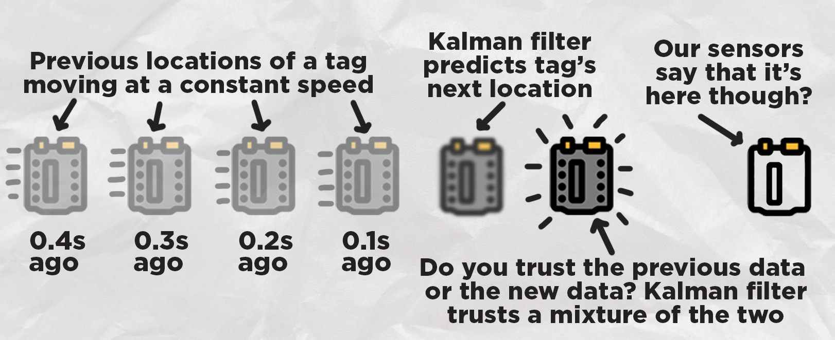
The Kalman filter works in two simple stages; it predicts what is about to happen, and then it corrects its prediction based on new sensor data:
The prediction stage uses variables for things called "states". These "states" just hold information from the last measurements. In our code, these states just store information about the position of the tag, and the speed of the tag (in x,y,z, so there are 6 in total). If you know where the tag was previously and what speed it was moving at, you can guess where it is going to be now! And this is what our prediction step does, it looks at the states from the last measurements, gets the location, gets the speed, and then predicts where it would be now.
The next stage is the correct stage. Our code is only predicting the next step every 0.1 seconds. Now our prediction is going to be accurate if the tag is moving at the same speed that it was 0.1 seconds ago, but what if it is speeding up? This is where we correct it. The rest of our code gets the distance measurements from the base stations, uses least squares to get the new location, and then the Kalman filter takes this new and raw data to make the correction. All it really does is that it takes the position that it predicted the tag to be in, and moves it slightly toward where the new data says it is. Once we have corrected our prediction and are happy with the location, we will update the states to start this cycle over again!
How much do we trust the prediction? How much do we trust the new measurement data? Well, that is the beauty of the Kalman filter, we get to choose. In the code, you will find two values of "Q" and "R" (towards the top of the SimpleKalman class):
        self.Q = 0.12
        self.R = 1.1
        self.dt = 0.10
These two values are the knobs that we can use to tune this correction stage. If you lower the Q value, you will tell the Kalman filter to trust the prediction more. If you lower the R-value, you are telling the Kalman to trust the newest measurements more. Out of the box, this code is tuned with Q fairly low, meaning that the system trusts the predictions a lot more. This gives us an incredibly smooth motion coming from the filter, but it means that is sluggish and less responsive as it needs a lot of new measurements to be pulled in a certain direction.
If you need a more responsive system, you can increase the value of Q (or decrease R), which will make the Kalman trust the newest measurements more. But this is a double-edged sword, as you will trust incorrect measurements more. The new and raw data is going to have noise in it, meaning that it will jitter around, and you should have seen this jitter in the red dot in all the visualisations. This noise or jitter is just a part of existing in the real world and is the main reason that entire fields of math and engineering have been dedicated to developing things like the Kalman filter.
And that is the entire idea behind tuning. You want to tune your values to trust the prediction enough that you get a smooth output to eliminate this jittery noise, but you also want to trust the newest data enough so that it is still responsive and doesn't "lag" behind too much. There is no fixed solution here or magic number; every project and every application will be different, and so you will need to tune it accordingly (also, it is pretty fun to do so).
And with that, you now understand how a simple Kalman filter works. However, that is the easy part; the hard part is writing the code to apply it in your project. If you are mathematically inclined, William Franklin has a great explanation of the maths behind this filter, and it is a great start in applying it to other projects. Another great source is LLMs like ChatGPT and Claude. These LLMs are very well-versed in simple Kalman filters, and if you paste in your project code, they should be able to help you implement one - all you need to do then is understand what's going on and how to tune it.
Where to From Here?
With that, we now have a system that can track a tag in 2d or 3d space - an incredibly powerful ability to have in a modern maker project. Even a decade or two ago, a system like this would be in the thousands, if not 10s of thousands of dollars and be difficult to access outside of a research lab or large organisation. But now, you can build this system with relatively inexpensive off-the-shelf maker-tier hardware - how incredible!
There are many ways to take this to the next level. If you placed an IMU on your tag, you could not only get the position of an object, but also its angle or orientation. The math we used in this demo guide could also be improved. We used a least squares + simple Kalman filter method as it gave satisfactory results, while still being somewhat beginner-friendly and able to run on a microcontroller. If you are chasing more accurate tracking, this code could easily be modified with the help of an LLM like ChatGPT or Claude to implement some more advanced tracking math.
If you do make anything cool with this though, or you need a hand with anything covered in this guide, feel free to post about it on the forum below. We are all makers over there and happy to help! Till next time though, happy making!

