I had been captivated by the sound levels of trains I could hear passing by Metford throughout the day/night. I wondered if a sound level sensor reporting data back over LoRa would help me understand when a train was noisy. I also like the idea of seeing or visualising a problem, in this case, an ambient sound level. As you deconstruct a problem it consists of information & that information consists of data. As such, if I could create sound level data & build that sound level data into visual sound level information, then I could perhaps better understand the problem. I also intended to deploy several devices to the field to try and detect the difference in sound levels of a common event at different distances/environments.

Overview:                                                                                                                                        

• Let’s begin…                                                                                                                                  
• The Hardware                                                                                                                         
• Version 1 (hardware listed above)                                                                                       
• Version 2 (hardware same as above, except for microphone)                                            
• Pycom Documentation                                                                                                         
• The sensor - Mic Amp, MAX 4466                                                                                       
• The IDE                                                                                                                                       
• LoRaWAN                                                                                                                                 
• The Things Network TTN                                                                                                         
• Our decoder code                                                                                                               
• Node-Red                                                                                                                                  

Literature Readings/Topics:                                                                                                       

• Sampling theorem                                                                                                                    
• Nyquist frequency                                                                                                                     
• Sample rate                                                                                                                              
• Bit depth                                                                                                                                    
• Sound pressure level                                                                                                                
• Decibel definition                                                                                                                      
• A weighted sound pressure level                                                                                             
• Fletcher Munson effect                                                                                                             
• Sound level as a function of frequency                                                                                    
• The Definitive + longer read, which covers pretty much everything                                     
• Sound bandwidth                                                                                                                      
• Filter bandwidth                                                                                                                        
• Analogue filter                                                                                                                           
• OP amp audio filtering                                                                                                              
• Digital to analog signal to noise ratio                                                                                       

Overview:

This project was a rapid prototype that myself (Andrew Stace) and Alistair Woodcock created for the Lake Macquarie Smart Neighbourhood Challenge (September 2018). Our main goal was simply to explore LoRa technology and found out how hard/easy it was to create a:

1. A sensor that records data.
2. Send that data over a LoRaWAN (The Things Network, TTN)
3. Get that data off the TTN & persist it in a database (MongoDB).
4. Export that persisted data to be used in a simple web-based front end.

Personally, I had been captivated by the sound levels of trains I could hear passing by Metford throughout the day/night. I wondered if a sound level sensor reporting data back over LoRa would help me understand when a train was noisy. I also like the idea of seeing or visualising a problem, in this case, an ambient sound level. As you deconstruct a problem it consists of information & that information consists of data. As such, if I could create sound level data & build that sound level data into visual sound level information, then I could perhaps better understand the problem. I also intended to deploy several devices to the field to try and detect the difference in sound levels of a common event at different distances/environments.

LoRa seemed like a good network option, given:

• The train lines are a couple of KMs away.
• I wanted to deploy several nodes across a large geographic area (significantly greater than a WiFi coverage).
• I wanted live data, not some kind of manual import process.

Already there was this awesome tutorial, Your First LoRaWAN Node on The Things Network. This tutorial really helped bootstrap our confidence that getting into this was more possible than not. I also wanted to continue where Chris finished. At the end of his tutorial he wrote,

“... Next, we'll look at turning bytes back into JavaScript Object Notation (JSON) for integration with a platform that can make all our devices work together. A platform like Node RED ...”

Along the way, the toughest things for us (everyone is different) was building the sensor, the electronics. Both Alistair & I are quite ignorant when it comes to electronics. But Alistair & I have web developer backgrounds. So we’ve both spent a large part of our life crushing our ego with problem-solving. As such, we were able to logic our way through most of the problems. It also helped to be able to rubber ducky our problems as we went.

In particular, the analog to digital conversion jazz was a bit tricky & using mean instead of average for our sampling (thank you Graham for the workshop where you provided that little insight) helped improve our data.

The more we got into it the more the science started to intrigue me. What actually is sound?! I was lucky enough to stumble into two engineers from SwitchedIn at the Newcastle Makers Festival, shout out to Sam Ireland & Sergio Pintaldi. They’re both really great guys and they eviscerated me on some of the science that’s behind the project. It really gave me a lot more to think about, which was awesome.

Sam, in particular, provided me with a list of literature topics to go out and explore. Upon which I’ve since tried to reduce each of the topics down into TLDR summaries (listed at the end of the notes). The TLDR summaries should be enough to allow you to think a bit more clearly about the science. But they certainly not enough to allow you to be competent when it comes to sound engineering.

Let’s begin…

Again, we’re assuming that you have already completed or attempted this tutorial Your First LoRaWAN Node on The Things Network

This project will take up where that tutorial finishes off. However, this won’t necessarily be a tutorial, meaning that it won’t be a step by step guide. It’s more so a compilation of our project notes & references which we found helpful along the way. There’s an implicit step by step logic in how we’ve ordered our notes, but we have left quite a bit of the thinking up to you. Where possible we will try to share code. However, more so we want to share our experience & notes we collected along the way. Hopefully, some of our notes OR the resources that we have attached to this project will help you solve some of the problems you encounter on your own project(s).

To begin we will look at the hardware which we started with…

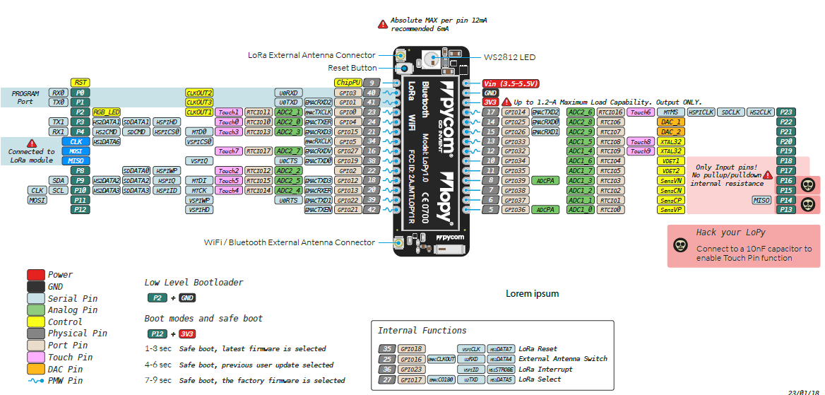
The Hardware:

• Baseboard: Pycom Expansion Board 3.0 
• Network access: Pycom LoPy4 (LoRaWAN)
• Antenna: Pycom LoRa & Sigfox Antenna Kit 
• Prototyping breadboard: Solderless Breadboard - 300 Tie Points (ZY-60) 
• Microphone: Electret Microphone Amplifier - MAX4466 with Adjustable Gain 

This kit, minus the microphone ended up becoming the kit which most entrants in the Smart Neighbourhood Challenge received to implement their project. It seemed like the logical thing to use as there was already a tutorial which used the pycom stack, given this, it massively helped bootstrap how to get connected on TTN. This meant less time getting connected, more time to focusing on getting data from a sensor, persisting it into a database & exposing that data via an API for a website to use.

Version 1 (hardware listed above)

+     It also has the light sensor on it as well 

Version 2 (hardware same as above, except for microphone)

This version was designed because it let us play around with bringing the device costs down.  Saved about ~$5 (not worth it financially, but from an educational point of view it was good).

Generally speaking, reading through all of the Pycom documentation gave us a good ballpark to work with & it’s very recommended that you put aside an hour to go through it and become generally familiar with all of the topics covered in their documentation. For example, we were able to pre-empt that ADC values would be a bit of a thing. But going through each of the things took a bit longer than we anticipated. The biggest issue was the pin mapping. This significantly slowed us down.

Because we are newbs when it comes to circuits, we used the following other projects as sources of inspiration:

• Potential adaptation: Pycom I2C Tutorial
• A sensor library example: Pycom Sensor Library Tutorial
• Mutate the LED: Pycom RGB LED Tutorial

Given our sensor (mic) was creating an analog signal, we needed to connect it to an analog pin. That wasn’t even clear to us when we first got into this. But after a bunch of research & experimentation, we sorted it out. The trick was to use the LoPy4 pinouts, not the Pycom Expansion board 3.0 pinout. Even then it wasn’t totally clear how GPIO36 related to P13, which was also G5. /shrug?!

I certainly think there’s room to improve the intuitiveness of the pinouts, &/or more likely Alistair & I were just too unfamiliar with reading pinout diagrams. In which case the whole industry needs to make pinouts more intuitive.

Here’s the list of resources we went through to understand the pinouts.

• Pycom Expansion Board Pinout
  
• Pin Mapping Help for Pycom
  
• Pycom Lopy4 Pinout  

Okay, so we knew how to read data from a sensor and print it out to console. Now it was time to really focus on our sensor & understand the data it was printing to console.

The sensor - Mic Amp, MAX 4466

Microphone sensors are trickier than light sensors. We eventually figured out we could use a light sensor as a validation or proof sensor, as it also produced an analog to digital signal. The reason we opted for this was that it wasn’t obviously clear to us what the ADC print out meant.

• Ok sure we got a value of 4096, but why?
• Ok, so 4096 is the biggest number a 12-bit data type can store.
• Ok, so our mic is maxing out, by why?
• Is our circuit broken? Is our mic truly maxing out? Surely it’s the former more than the latter.
• If our circuit is broken, how do we fix it? If we fix it, how can we tell that we’ve fixed it? Are we sure that we’re using the correct pin etc...

Given this lack of confidence, we were able to offset our uncertainty with the light sensor. As it’s very easy to control the amount of light that a light sensor receives. This means that we can do more accurate correlation/causation tests as we work through our problems. Put another way, we were certain that we were now using the right pin. Which pretty much meant that our mic circuit wasn’t correct. As such, we were able to conclude that our microphone sensor was indeed working, but the mic’s signal was getting too much “noise” or as we presumed voltage and it just kept giving us a reading of 4096 to console.

With the assumption that the signal had too much voltage, we figured that the way to get less voltage is by adding resistance (again, we’re proper newbs when it comes to electronics). Thus we decided to bring the voltage back by using a resistor. We tried a 3k ohm resistor, but no dice. We then chucked a 10k ohm resistor in front of the power and this reduced the (voltage) noise & created a more stable reading. We now started to see data readings which weren’t just 4096. This was a really great moment for us when we could see sound correlating with our console out. Here is the video we have from that moment :)

This understanding took several hours to figure out, but we were also still sceptical of the actual audio that the microphone is picking up. It looked like we had sound levels correlating with music we played etc. But still, were we detecting lots of low-frequency sound or high-frequency sound? What was the sound like that we're hearing on the mic? The correlation looked pretty loose, but certainly, that’s probably an artefact of our sampling as well. Things were starting to get more complicated but in a good way.

Other issues came into calibrating the mic’s ADC reading to dB (on a smartphone) & background noise (children, cars, misc).

Given we can produce an ADC value from the light sensor, we used that as the initial sensory element that we transfer over LoRa. Meanwhile, we continued to look into understanding the microphone sensor. This allowed us to continue onto the LoRaWAN aspects & come back to the mic sensor.

In the end, we didn’t convert our sound level reading into dB, as we weren’t satisfied with the quality of the mic/data. We did end up sending the sound level data over LoRa, but it wasn’t converted to dB before we sent it. For the most part, this just has us thinking about what changes we can make to get better data, to do a better conversion of the sound level data. Perhaps we could keep the client application more lightweight and do the conversion as it came into TTN, or perhaps we could simply convert the data as we imported or exported it from the DB. Many ideas are on the table, but the most important ideas circled improving the mic sensor design.

Example circuits which we originally based our sensor on:

• Arduino Sound Level Measurement
  
• Adafruit Microphone Amplifier Breakout Assembly and Wiring 

 

• Pycom Documentation Syntax
  
• Pycom Wipy Machine ADC
  
• Pycom Tutorials ADC
  
• Pycom Tutorials Firmware API Machine ADC
  

• https://www.youtube.com/watch?v=SToBPCajwc0

 

• Note: Currently time is starting at unix epoch (we’re guessing because no network time setup has occurred)
• Syncing to RTC to Network Time
  

The IDE

At this point, we’ve moved pretty quickly through our hardware & skipped quite a bit of some of the other parts of our project. So let's also quickly talk about our IDE.

The IDE we used was Atom. In particular, we also installed the Teletype package which was a great way to cowork. It also setups a great way to work remotely as well. One person authors a file & the other person can collab on it. Talking to the Pymakr varies between different operating systems, so perhaps connecting it to WiFi would have improved compatibility; however, we were both developing on Mac & we only ever left it plugged into the one Mac laptop.

Steps for installing Atom on a Mac:

• Install IDE: Atom IDE
  
• Install Atom packages:
• Install Teletype (collaborating on code) => https://teletype.atom.io
• Install Atom Shell Commands
• Create a Project Folder
• Login to Atom Teletype
• Setup a GitHub account
• Share your Project Folder
• For example: atom://teletype/portal/174a25f5-2d3d-4b76-8b96-7a8475e2b8dc
• Install Pymakr package (version, 1.4.2 : date, 15.09.18), https://docs.pycom.io/g ettingstarted/installation/pymakr
• Getting started with PyCom, https://docs.pycom.io/
• Connect Pymakr board to a computer via USB (assuming Mac)
• Connect to your Pymakr board via the Atom IDE Pymakr interface

■     Look up com ports, serial interfaces etc…

■     For example, open up a terminal and run the command

• ls /dev/tty.*

■     Update your pymakr.conf to talk with the write serial interface.

 

We now have some data printing out to our IDE’s console. We now need to get that to transmit over LoRa. We will be light on the steps involved here, as there are other tutorials which cover how to get data onto a LoRaWAN (TTN).

Summary: see other tutorials

• LoRaWAN Over The Air Authentication (OTAA): https://docs.pycom.io/tutorials/lora/lorawan-otaa
• AS923 VS 915

○     https://www.thethingsnetwork.org/forum/t/can-australian-users-agree-on-using-a-single-frequency-plan/17660

Summary: see other tutorials

Create an account

• https://console.thethingsnetwork.org/

Decoding:

1. Before we transfer our sensor data onto TTN we need to put data into byte form and/or hex form.
1. Because our sensor data was producing readings of an integer value from 0 to 4096. We only need a possible 12 bits to explain this data value.
2. The minimum we can send is in a byte which is 8 bits.
3. However, a hex-digital is 4 bits. So technically we only need 3 hex-digits to represent our data (3 x 4 = 12 bits).
2. TTN receives the raw hex version of our data & we need to decode (unhexify) it.
1. We’ve pulled some of the decode functionality from this repository and put it into the decoder javascript file on TTN
   https://github.com/thesolarnomad/lora-serialization
   We’ve also used the c files reference for how to format the data we send from python.

Our decoder code

In order to use this decoder code, we strongly recommend you spend a bit of time understanding base 2 (binary), base 16 (hex), bits & bytes. It seems like a semi-complicated thing, but honestly stopping and spending a little bit of time to understand binary/hex will help you in so many other areas of computing.

 

var bytesToInt = function(bytes) {

  var i = 0;

  for (var x = 0; x < bytes.length; x++) {

    i |= +(bytes[x] << (x * 8));

  }

  return i;

};

 

var unixtime = function(bytes) {

  if (bytes.length !== unixtime.BYTES) {

    throw new Error('Unix time must have exactly 4 bytes');

  }

  return bytesToInt(bytes);

};

unixtime.BYTES = 4;

 

var uint8 = function(bytes) {

  if (bytes.length !== uint8.BYTES) {

    throw new Error('int must have exactly 1 byte');

  }

  return bytesToInt(bytes);

};

uint8.BYTES = 1;

 

var uint16 = function(bytes) {

  if (bytes.length !== uint16.BYTES) {

    throw new Error('int must have exactly 2 bytes');

  }

  return bytesToInt(bytes);

};

uint16.BYTES = 2;

 

var latLng = function(bytes) {

  if (bytes.length !== latLng.BYTES) {

    throw new Error('Lat/Long must have exactly 8 bytes');

  }

 

  var lat = bytesToInt(bytes.slice(0, latLng.BYTES / 2));

  var lng = bytesToInt(bytes.slice(latLng.BYTES / 2, latLng.BYTES));

 

  return {lat: (lat / 1e6), lng: (lng / 1e6)};

};

latLng.BYTES = 8;

 

var decode = function(bytes, mask, names) {

 

  var maskLength = mask.reduce(function(prev, cur) {

    return prev + cur.BYTES;

  }, 0);

  if (bytes.length < maskLength) {

    throw new Error('Mask length is ' + maskLength + ' whereas input is ' + bytes.length);

  }

 

  names = names || [];

  var offset = 0;

  return mask

    .map(function(decodeFn) {

      var current = bytes.slice(offset, offset += decodeFn.BYTES);

      return decodeFn(current);

    })

    .reduce(function(prev, cur, idx) {

      prev[names[idx] || idx] = cur;

      return prev;

    }, {});

};

 

function Decoder(bytes, port) {

  var decoded = {};

 

  if (port === 1 || port === 2) {

   

    decoded = decode(bytes,

      [ uint16,  uint16, latLng],

      ['light', 'sound', 'pos']

      );

   

  }

  return decoded;

}

 

Thus far we’ve covered the hardware, our IDE, LoRaWAN & TTN. It should be possible for you to use the notes thus far to have your hardware print out data to console & more so, you should be able to see that data being transmitted onto TTN. Let us know if you would like us to add more details or steps to any of the above section.

Ok, so it’s nothing short of amazing to see your data’s bits transfer wirelessly over KMs on LoRaWAN. But in my opinion, Node-Red is where I really engage a heavy-breathing-cat.jpg. As Node-Red (in my opinion) has a massively wider use case. Meaning that the power to make things quickly in Node-Red & for them to just work has awesome potential.

 

But let’s keep focused, why Node-Red!? Well we have data in the TTN, but now we need to:

• Get that data &
• Do stuff with it

The stuff we want to do is persist it (store it in a database). The other stuff we want to do is access it up when we want & display it in some nice visual way.

To persist it we chose MongoDB. In order to explain why MongoDB, it’s easier to say, why not MySQL or MSSQL etc. A lot of people are more familiar with relational databases like MySQL/MSSQL etc. The problem with relational databases is that you need to setup what your tables will look like, not hard, but it’s a thing. What columns there will be and what data types will be stored in those columns etc.

• On one hand, you can be thinking to yourself, well I just want to store an integer or a float value. That’s all I’m transmitting onto TTN.
• Ok great, so go create your table with an ID auto incrementing as a key and another column to store the integer or float etc.
• But now you want to send another type of data from your device.
• Ok easy, update the code on the node/sensor to send another type of data. Confirm it’s being decoded on TTN. Now update your table to have the new column to store this new data type.
• Ok done, easy.
• Now you don’t want it anymore.
• Undo the above steps etc, blah blah blah.

This uncertainty about what you want to send or store is a perfect case for a document database. A document will just accept any new data you throw at & that can change between each document without you doing anything.

Consider again that we want several devices/nodes out there in the field transmitting data, will each of these be transmitting the exact same data & having it persisted (maybe, probably… but more importantly, what if we didn’t need to care, not yet anyway, not while we’re prototyping this).

Our sensors/nodes can transmit varying packets of data onto TTN & we can use Node-Red to observe that data. Then we can store that data into a document without caring too much about it includes. Of course, there are no free lunches and we will need to care about the data when we go to display it, but the upside benefit is greater than the downside cost of dealing with the potentially inconsistent data.

But the point I’m trying to make here is that MongoDB gives us a very flexible option for persisting our data. It means that we don’t need to spend ANY time updating database tables as we rapidly prototype this thing. We simply see the data on TTN & then store it. The next package of data arrives & it’s got more or less data than the previous one, who cares, it simply gets stored.

Anyway, enough about databases let’s get onto installing Node-Red. In our case we were installing Node-Red on Ubuntu 16.04, running on a Udoo x86. It’s basically a Raspberry Pi on steroids. https://www.udoo.org/udoo-x86/

Again this isn’t a step by step tutorial, so we have captured our notes from this step & kept the resources we used to setup Node-Red on our device. For example, we got install issues when we tried to add ‘npm i node-red-contrib-ttn’.  The first guide (see below) expresses to use node-legacy, as there are conflicts with node & nodejs environmental variables.

There’s a simple workaround to create a symbolic link from nodejs to node (see below). You can install nodejs, not node-legacy.

On Ubuntu 16.04 installing nodejs or node-legacy will only give you 4.2.5. This version of node will allow you install Node Red. But once Node-Red is installed you won’t be able to install it’s TTN plugin. Therefore, you also need to install an npm package called ‘n’. ‘n’ allows you to install different versions of nodejs very easily. Once you’re on a more recent version of nodejs/node, the Node-Red TTN addon will install.

• https://www.digitalocean.com/community/tutorials/how-to-connect-your-internet-of-things-with-node-red-on-ubuntu-16-04
• https://www.digitalocean.com/community/tutorials/initial-server-setup-with-ubuntu-16-04
• ubuntu- https://www.digitalocean.com/community/tutorials/how-to-install-nginx-on-ubuntu-16-04
• https://www.digitalocean.com/docs/networking/dns/
• https://www.digitalocean.com/community/tutorials/how-to-secure-nginx-with-let-s-encrypt-on-ubuntu-16-04
• sudo ln -s /usr/bin/nodejs /usr/sbin/node
• sudo npm install -g n
• sudo    n latest OR sudo n 8.9.0 OR sudo n lts (ETC)
• we went with lts
• https://nodered.org/
• https://www.youtube.com/watch?time_continue=35&v=vYreeoCoQPI
• https://flows.nodered.org/flow/a14cfb633c0bd093d52cab3c12297ee9
• https://www.npmjs.com/package/node-red-contrib-ttn
• https://nodered.org/docs/getting-started/adding-nodes

https://github.com/TheThingsNetwork/nodered-app-node/blob/HEAD/docs/quickstart.md

We should now have Node-Red installed & we should now have the TTN palette added. This means that we can use Node-Red to observe the data flowing into our TTN application or specifically from our TTN application’s devices.

Now even though I made a lot of noise about MongoDB. It appears as though I didn’t record any notes for installing it or getting it working in Node-Red. Perhaps because it was easy enough to install without a problem using Google searches:

• “Install mongodb ubuntu 16.04”
• “Node red mongodb”

Off the top of my head, there was something about different mongodb versions & how there were multiple mongodb palettes in Node-Red. But nothing that was problematic/difficult to overcome. Suffice to say, once you have Node-Red up and running & it’s talking with TTN, then persisting the data is pretty straightforward.

Now we have our data persisted. The next thing we want to do is use Node-Red to create an API or URL that we can hit that we will return our documents/data back as JSON. Quickly I think you’ll find that Node-Red makes tasks like and may others trivially easy. As such it’s not difficult to set up the URL which returns this data as JSON. This is what our Flow looked like once “complete”. (nothing is ever complete)

 

Now that we had this data it was just a matter of creating an interface/view to display the data. The code is seriously terrible as it was thrown together late one night. But you can view it on http://soundscape.ena.digital/

 

You will notice that the data won’t often load. That’s because Node-Red & MongoDB, running on my Udoo x86 is usually powered off. That said, you can still read through the page's source and see how we access the JSON data & then display it into a table using chart.js.

That’s pretty much were our sound sensor project finished up by the time we submitted it for the Smart Neighbourhoods challenge. We were able to do most of this in a weekend (in a hackthonesque timeframe), with most of the work happening on Saturday. Of course, there were a couple of hours here and there before and after the weekend. But the most impressive thing we got from this project was how quickly you could throw together something and get it to work.

If we look at what we achieved in this project, we:

1. Prototyped hardware which could hear sound, turn that sound into a value.
2. Send that value over LoRaWAN via The Things Network.
3. Store that network data into a database.
4. Retrieve that data from the database.
5. Fetch data from the database incrementally & show live updates of the sound value that we were transmitting over TTN/LoRa.

In essence, we had set out what we wanted to achieve, albeit the todo list was still quite long.

• Timecoding our dataset.
• Add alerts to our respond to our dataset.
• Data wasn’t reliable/accurate, as the mic/sensor wasn’t reliable.
• Data sampling / processing of could be improved.
• Power utilisation/optimizations, there’s no power cycling, device is always on.

In order to get it to work better or improve it, well, that’s somewhat more of an exponential curve to overcome (see literature reading section below). But worth noting, the beauty of scientific literature is that everything is reducible to fairly simple concepts, albeit many simple concepts needing to be understood. This means that with enough time & persistence we can certainly understand many of these simple things & as such a few of the complicated things.

3) Graham from Core Electronics also had an awesome idea, similar to (2.a) where the nodes cooperate and coordinate a listen/get ready function. Where LoRaWAN data transfer could likely travel faster than the speed of sound. Thus you could listen at a perimeter device & then have other devices begin to get ready for an incoming sound.

Literature Readings/Topics:

Sampling theorem

TLDR: Sound is the combination of a set of tones, where each tone has a certain frequency. Understanding the frequency of these sounds, lets us properly sample them, such that they can be reconstructed with accuracy. Take the maximum tone frequency within your set of sounds and sample it at a rate at least twice its frequency.

A note on the maths side of this jazz, we have a signal, and from the signal, we produce a spectrum. The spectrum allows us to realise the maximum frequency value. We then double that max frequency value to give us the Nyquist rate. There’s still a bunch of maths jazz involved that we have deferred, such as actually running through the equations between the spectrum and the signal.

Notes:

“A bandlimited signal can be reconstructed exactly if it is sampled at a rate at least twice the maximum frequency component in it.” https://nptel.ac.in/courses/106106097/pdf/Lecture08_SamplingTheorem.pdf

Bandlimited signal:

Bandlimiting is the limiting of a signal's frequency domain representation or spectral density to zero above a certain finite frequency. A band-limited signal is one whose Fourier transform or spectral density has bounded support.

https://en.wikipedia.org/wiki/Bandlimiting

Fourier transform:

The Fourier transform decomposes a function of time into the frequencies that make it up, in a way similar to how a musical chord can be expressed as the frequencies of its constituent notes.

https://en.wikipedia.org/wiki/Fourier_transform

Spectral Density:

The power spectral density (PSD) of the signal describes the power present in the signal as a function of frequency, per unit frequency. Power spectral density is commonly expressed in watts per Hertz (W/Hz).

https://en.wikipedia.org/wiki/Spectral_density

 

Frequency component:

An example is the Fourier transform, which converts a time function into a sum or integral of sine waves of different frequencies, each of which represents a frequency component. The 'spectrum' of frequency components is the frequency-domain representation of the signal.

            https://en.wikipedia.org/wiki/Frequency_domain

Nyquist frequency

TLDR: Read above sampling theorem notes; + the Nyquist frequency or Nyquist rate is the minimum required sampling rate. Which as we know from above, is 2 times the tone’s maximum frequency.

The minimum required sampling rate fs = 2fm is called Nyquist rate

https://nptel.ac.in/courses/106106097/pdf/Lecture08_SamplingTheorem.pdf

Playing with logic, not maths, we can simply ask, what is the audio range of the human experience? 20 to 20000 Hz. Ok, so we can simply double 20000 Hz and come up with a Nyquist rate of 40000 Hz, or 40 kHz.

Sample rate

TLDR: The number of audio samples taken per second, measured in Hertz, or kiloHertz. 1 sample per second = 1 Hz.

The sample rate is the number of samples of audio carried per second, measured in Hz or kHz (one kHz being 1 000 Hz). For example, 44 100 samples per second can be expressed as either 44 100 Hz, or 44.1 kHz. Bandwidth is the difference between the highest and lowest frequencies carried in an audio stream

https://wiki.audacityteam.org/wiki/Sample_Rates

Bit depth

TLDR: Bit depth acts as the possible resolution that a signal can be sampled at. Every time a signal is sampled, the sample must be stored in digital form. Its digital form has a maximum potential size, which is understood by the bit depth. For example, a bit depth of 12 bits, has a range of 0 to 4095 integer values or 4096 possible values. Think about how precise a sample could be when there’s only that much room to store the digital values.

https://en.wikipedia.org/wiki/Audio_bit_depth

Sound pressure level

TLDR: Sound waves propagate through space and create different pressures for different sounds. The measurement of sound is impacted by the pressure levels of the environment. The measurement of the sound pressure level is done in decibels. 

Notes:

SPL is actually a ratio of the absolute, Sound Pressure and a reference level (usually the Threshold of Hearing, or the lowest intensity sound that can be heard by most people). SPL is measured in decibels (dB), because of the incredibly broad range of intensities we can hear.

http://www.nchearingloss.org/spl.htm?fromncshhh

Sound pressure level (SPL) or acoustic pressure level is a logarithmic measure of the effective pressure of a sound relative to a reference value.

https://en.wikipedia.org/wiki/Sound_pressure#Sound_pressure_level

The lower limit of audibility is defined as SPL of 0 dB, but the upper limit is not as clearly defined. While 1 atm (194 dB Peak or 191 dB SPL) is the largest pressure variation an undistorted sound wave can have in Earth's atmosphere, larger sound waves can be present in other atmospheres or other media such as underwater, or through the Earth.

Equal-loudness contour Ears detect changes in sound pressure. Human hearing does not have a flat spectral sensitivity (frequency response) relative to frequency versus amplitude. Humans do not perceive low- and high-frequency sounds as well as they perceive sounds between 3,000 and 4,000 Hz, as shown in the equal-loudness contour. Because the frequency response of human hearing changes with amplitude, three weightings have been established for measuring sound pressure: A, B and C.

• A-weighting applies to sound pressures levels up to 55 dB,
• B-weighting applies to sound pressures levels between 55 dB and 85 dB,
• and C-weighting is for measuring sound pressure levels above 85 dB.

 

In order to distinguish the different sound measures a suffix is used: A-weighted sound pressure level is written either as dBA or LA. B-weighted sound pressure level is written either as dBB or LB, and C-weighted sound pressure level is written either as dBC or LC. Unweighted sound pressure level is called "linear sound pressure level" and is often written as dBL or just L. Some sound measuring instruments use the letter "Z" as an indication of linear SPL.

https://en.wikipedia.org/wiki/Sound_pressure#Examples_of_sound_pressure

Decibel definition

TLDR: see sound above about sound pressure level; + given a sound wave is a set of varying pressures, decibels is the mapping of those pressure to a logarithmic scale.

The decibel (symbol: dB) is a unit of measurement used to express the ratio of one value of a physical property to another on a logarithmic scale.

https://en.wikipedia.org/wiki/Decibel

decibel ˈdɛsɪbɛl’

A unit used to measure the intensity of a sound or the power level of an electrical signal by comparing it with a given level on a logarithmic scale.

(in general use) a degree of loudness. "his voice went up several decibels"

A weighted sound pressure level

A-weighting is applied to instrument-measured sound levels in an effort to account for the relative loudness perceived by the human ear, as the ear is less sensitive to low audio frequencies. ... It is also used when measuring low-level noise in audio equipment

https://en.wikipedia.org/wiki/A-weighting

Fletcher munson effect

TLDR: The human experience hears sound waves of different frequencies, at different levels of loudness. Loudness is measured in “phons”. For example, something of a very low frequency must be made comparatively louder than a sound of a higher frequency. But that said, “the loudness of a sound is not equal with its sound pressure level and differs for different frequencies”. Thus it’s not a given that a higher frequency tone, will directly equate to a higher amount of loudness.

1 minute explainer: https://www.youtube.com/watch?v=4moLvrH4QVM

12 minute explainer: https://www.youtube.com/watch?v=J7QPHXEBY80

The Fletcher–Munson curves are one of many sets of equal-loudness contours for the human ear, determined experimentally by Harvey Fletcher and Wilden A. Munson, and reported in a 1933 paper entitled "Loudness, its definition, measurement and calculation" in the Journal of the Acoustical Society of America

https://en.wikipedia.org/wiki/Fletcher–Munson_curves

Equal-loudness contour

            An equal-loudness contour is a measure of sound pressure (dB SPL), over the frequency spectrum, for which a listener perceives a constant loudness when presented with pure steady tones. The unit of measurement for loudness levels is the phone and is arrived at by reference to equal-loudness contours. By definition, two sine waves of differing frequencies are said to have equal-loudness level measured in phons if they are perceived as equally loud by the average young person without significant hearing impairment.

https://en.wikipedia.org/wiki/Equal-loudness_contour

Sound level as a function of frequency

TLDR: Sound level is the decibel (dB) representation of a tone or set of tones, relative to its sound pressure level. Where the sound pressure level is an indicator of a tones loudness to a normal human ear, in normal earth atmospheric conditions.

For example, a sound wave is measured in Pascals (Pa). But a sound level is expressed in Decibels (dB). Where Pa is the “actual measured sound pressure level”. But then this Pa value becomes a dB value by being referenced to something, such as the